Variable Selection Methods
This post will briefly introduce the concept of multicollinearity and variable selection methods as a remedy to address multicollinearity issues.
Multicollinearity
As a gentle introduction, let’s get a glimpse of the concept of multicollinearity by an example. As I am a huge fan of BTS, let’s imagine a situation where we have a dataset containing biological information about the member Jin and we are going to make a regression model on Jin’s health index. Among the dataset, we noticed that there are variables such as “width of eye”, “length of eye” and “color of eye”. Regarding these variables, it is reasonable to question the validity of these features as they all seem to be related to one common feature - “eye”. Intuitively, there’s gotta be some amount of information overlapped in them so we don’t necessarily need all these variables.
This is the issue of multicollinearity. By formal definition, it is said that multicollinearity exists when the (explanatory) variables are highly “correlated” to each other. In other words, this is very inefficient in terms of the information because we are using all the variables to unnecessarilry expend the dimension of our model whereas only a few subset of variables is sufficient. Increase in dimensionality often results in “curse of dimensionality”, hence a remedy is required.
Luckily, there are statistical methods which can possibly solve this problem and in this post, Variable Selection Method will be introduced.
Variable Selection
The objective of variable selection is to find subset of variables that are most “relevant” for prediction or equivalently, “important” in terms of the amount of information contained in them.
Our universe is sparse. Stretch out your hand in the air. Can you feel something? Although there are elements like oxygen in the air, we can’t feel them nor can we see them. Thus let’s only focus our attention to the matters we can directly interact with because you wouldn’t be likely to explain the total amount of oxygen in your room when you are asked by your friend to describe your room. Rather, what you will mainly be mentioning for description are the nitty-gritty details such as your recently bought PS5 or a fancy poster of Lionel Messi.
In this sense, when we are looking at a particular dataset, we always have to keep mind that we don’t necessarily need every information in the data because some variables are just too trivial or redundant. In statistics, these unimportant information often cause “noise” and by identifying only the relevant variables, we are able to reduce the noise contained in the data which can hopefully improve the performance of our estimator (or fitted model).
Then how can we select only these “relevant information”? The foremost and most straightforward way is by the rule of thumb. We can just exclude one variable from the model at a time, calculate and record the loss (mostly MSPE), compare the loss scores for each of the trials and select the best subset of variables that showed the minumum loss. Actually, when we use the software R and conduct regression analysis, R returns the best subset of variables by this method. This method is called as subset selection. The strength of subset selection is that it is very straightforward so it is easy to implement and it produces a model that is highly “interpretable” because the discarded variables can be interpreted as irrelavent.
However, subset selection has few serious drawbacks. Since it is a discrete process, meaning that variables are either selected or discarded, all of the information in the discarded variables is completely lost. Moreover, it often exhibits high variance so its performance tends to shrink when new data is provided.
In order to improve these apparent weaknesses, the so called shrinkage methods had been developed, which is said to be more continuous and don’t suffer from high variability as much as the subset method. The most famous shrinkage methods are Ridge Regression and Lasso Regression, so let’s take a brief look at each of them and their implementation in R.
Ridge Regression
For people familiar with linear regressions, let’s recall the normal equation, which is used to derive the regression coefficients (LSE) of linear regression models. Here is the formula.
Note that the regression coefficient beta can only be derived when the design matrix X is of full rank. When multicollinearity exists between the columns of a matrix, then that matrix is not full rank and we can’t derive the unique least squares estimate of beta.
In this situation, Ridge regression handles this problem by imposing a penalty on the size of the matrix to arbitrarily make normal equation solvable. Here’s the idea.
By adding λ to the left side of the normal equation, the matrix is forced to have full rank (or invertible equivalently). Here, λ is called as complexity parameter and it controls the amount of shrinkage, meaning that the regression coefficients of irrelevant variables converge to 0.
In ridge regression, the regression coefficients infinitely converge to 0 but doesn’t become exactly 0. Thus the larger the value of λ, the greater the amount of shrinkage. It can also be seen that the coefficients can be derived precisely in a closed form because it is a linear combination of matrix X and Y.
Also, the normal equation for ridge regression can be expressed explicitly in terms of the constraint as the last line of the equation above. Specifically, the constraint for ridge regression is the square of the norm of β, so this panelty is often called as L2 panelty. In this sense, as ridge regression sort of manages, or “regularizes” β to control variance, another name for ridge regression is L2 Regularization.


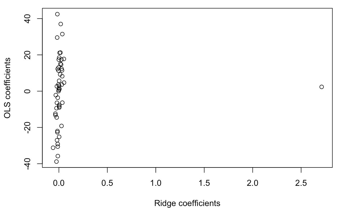
The graph above is a comparison between OLS (Ordinary Least Squares) coefficients and the ridge coefficients based on optimal λ suggested by R. Each regression was fitted on a randomly created data points from the multivariate normal distribution. The y-axis represents ordinary regression coefficients whereas the x-axis is ridge coefficients. It is clear that most of the ridge coefficients converged nearly to 0 while the coefficients are all over the place in the ordinary linear regression .
Thus by using Ridge Regression, we can discard variables that has ridge coefficient close to 0. This is one way of performing a variable selection.
Lasso Regression
Now let’s take a took at another famous shrinkage method called as lasso regression. The basic idea is similar to that of ridge regression, where the only critical difference is that lasso regression uses L1 panelty. In fact, lasso is an abbreviation for “Least Absolute Shrinkage and Selection Operator”. As its name explicitly suggests, lasso regression uses absolute panelty and although this might seem trivial, it creates a lot of difference and complexity compared to the ridge regression.
Because of the absolute panelty, the estimated coefficients $\hat \beta_{lasso}$ cannot be derived in a closed form since the normal equation is non-linear in X and Y. Hence for lasso regression, numerical optimization methods such as Newton Rhapson Method is used as a roundabout solution.

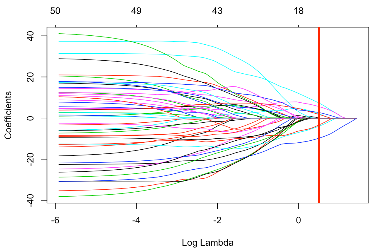
Above is the result of fitting lasso regression to the same data used in ridge regression. It can be seen that some of the coefficients have disappeared completely. This is because the absolute panelty of lasso regression makes the regression coefficients of “insignificant” variables exactly 0. It can be visualized as the following graph.

The x-axis corresponds to the log scaled values of λ, which is the shrinkage parameter that we discussed earlier and y-axis is the corresponding lasso coefficients. The vertical red line is the best λ suggested by R. It can visually be examined that for the best λ, most of the coefficients have become 0. We can then use this result as a guideline to exclude those variables in future analysis and modeling procedure.
As a last part of this post, let’s try to understand the difference between ridge and lasso regression in terms of geometrical aspect. Why is lasso regression able to make coefficients exactly 0 while ridge regression cannot?
Remarks
We have just conducted a variable selection! Keep in mind that the purpose of variable selection is to define only a subset of important variables to be used in further analysis. Therefore, variable selection itself is not the ultimate goal and is rather a first step in a complete statistical analysis procedure.
Although lasso and ridge methods can be used to reduce multicollinearity, variable selection methods have inherent limitations as they merely tell us which variables to be used or not. In other words, these methods are subordinated to the original data - they don’t provide any new insight or viewpoint of the data. Also, they are discrete processes like I mentioned, so there is no way of retaining information in the discarded variables.
In the following post, we will see how we can manipulate the data using dimension reduction methods.