Cluster Analysis

2020, Dec 06

 

This post will briefly introduce the concept of Cluster Analysis for defining clusters inside a dataset.

 

---

Cluster Analysis (CA)

In this post, we will be talking about Cluster Analysis.

Until now we have seen Principal Component Analysis and Factor Analysis to reduce dimensionality of the original dataset in terms of its variables. Both methods decompose data matrix by its column vectors to find a subset of variables that account for enough information of the original data. However, cluster analysis performs dimension reduction on observations, that is, by row vectors. This is the crucial difference that distinguishes Cluster Analysis from rest of the dimension reduction methods.

In other words, the goal of cluster analysis is to find groups of clusters that can “adequately” separate and group the observations. Since the word “adequately” is a little vague in its meaning, we can formally define its meaning as follows.

• observations inside the same clusters are similar as possible

• observations within different clusters are different as possible

   

---

Distance

However, the above definition is still somewhat ambiguous. How are we going to measure the similarity and dissimilarity of each observations? Here’s where the mathematical concept of distance comes in. To define distance, we foremost need a measure, and there are various definitions of different mathematical measures to define the distance between two objects.

 

 

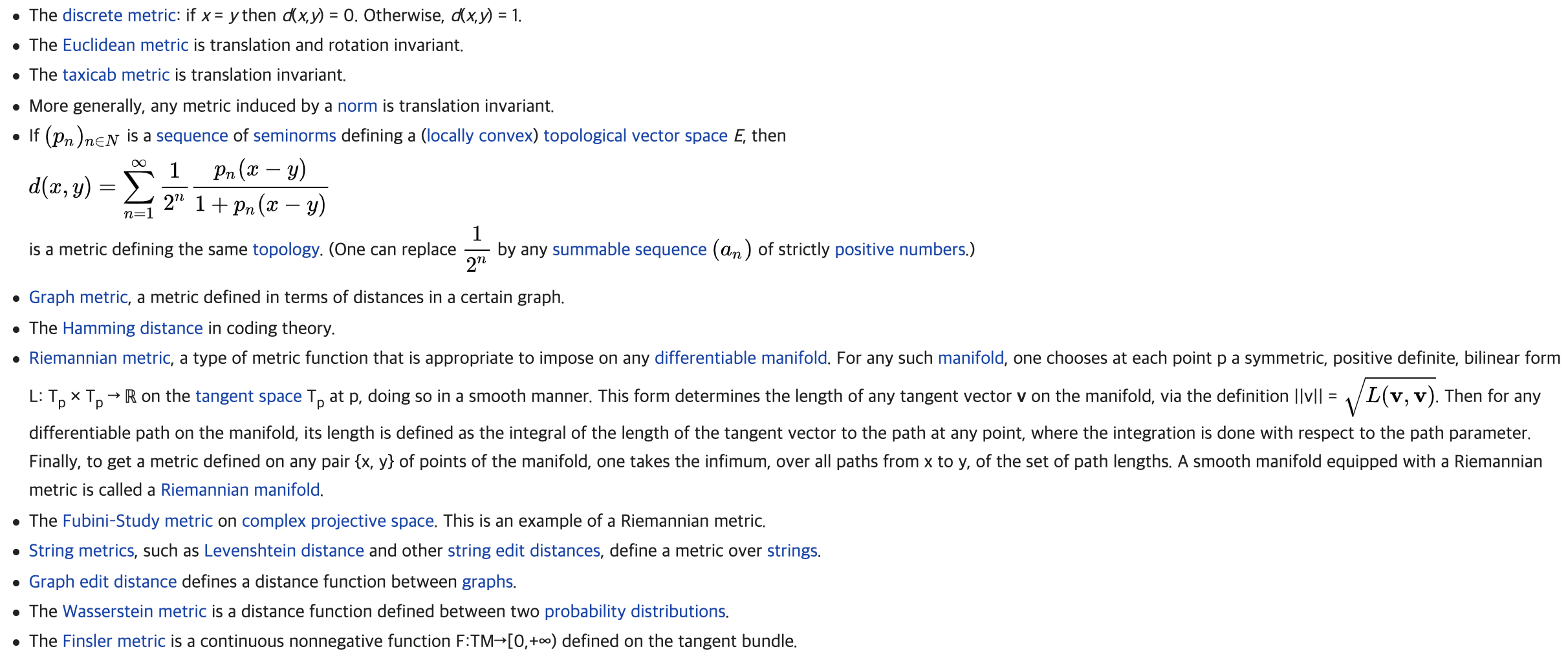
Above is an wikipedia example of list of different distances, but all of them are defined to accomplish one single purpose; to measure the “closeness” of objects. The “closer” the objects are, the more homogeneous or similar they are. Since going into the details of all of the distances above would be tedious and time consuming, let’s focus on some of the key points of distance and move on.

Normally when we think of distance between two things, we are mostly familiar with the “Euclidean Distance”, which is the most famous and widely used distance measure for calculating “physical distances”. Physical distance literally means the distance between two physical objects. We say Tokyo is around 1,150 km apart from Seoul. This is physical distance.

But it’s important to note that there also exists “psychological distance” as well. Like when we are asked, “How close do you think you are with your best friend?”, the answer is certainly not going to be something like “Oh, it’s about 10 meters”. In this situation, we need another measurement that can account for our psychological intimacy.

Likewise, the measurement of distance can vary according to the goal of our interest and the distance measure to be used for cluster analysis should also be different with respect to the nature of our data. Although most of the data we’ll face is going to be about physical properties, it is worth noticing that we should not blindly rely on the euclidean distance regardless of data environment.

 

---

K-Means Clustering

Anyways, let’s come back to our main topic. Now we are clear that cluster analysis is about grouping observations to make clusters. This process is done in a predefined order and principles, which is formally called as “algorithm”. There are lots of clustering algorithms and research is still ongoing.

In this post, we will use an algorithm known as “K-Means Clustering” which is the most widely implemented clustering methodology. The reason why it is named as “K-means” is because it makes clusters based on the mean of each clusters.

The steps of clustering for K-Means algorithm is the following.

 

1. Select number of clusters and distribute the observations accordingly
2. Calculate the centroid for each cluster (centroid is calculated as the mean of each cluster)
3. For each observation, calculate the within-group distances (distance between observation and the centroid)
4. Reallocate observations into the cluster whose centroid is the closest
5. If the cluster of any observation has changed, return to step 2 and repeat

 

As an illustration, these steps can be visualized as follows:

 

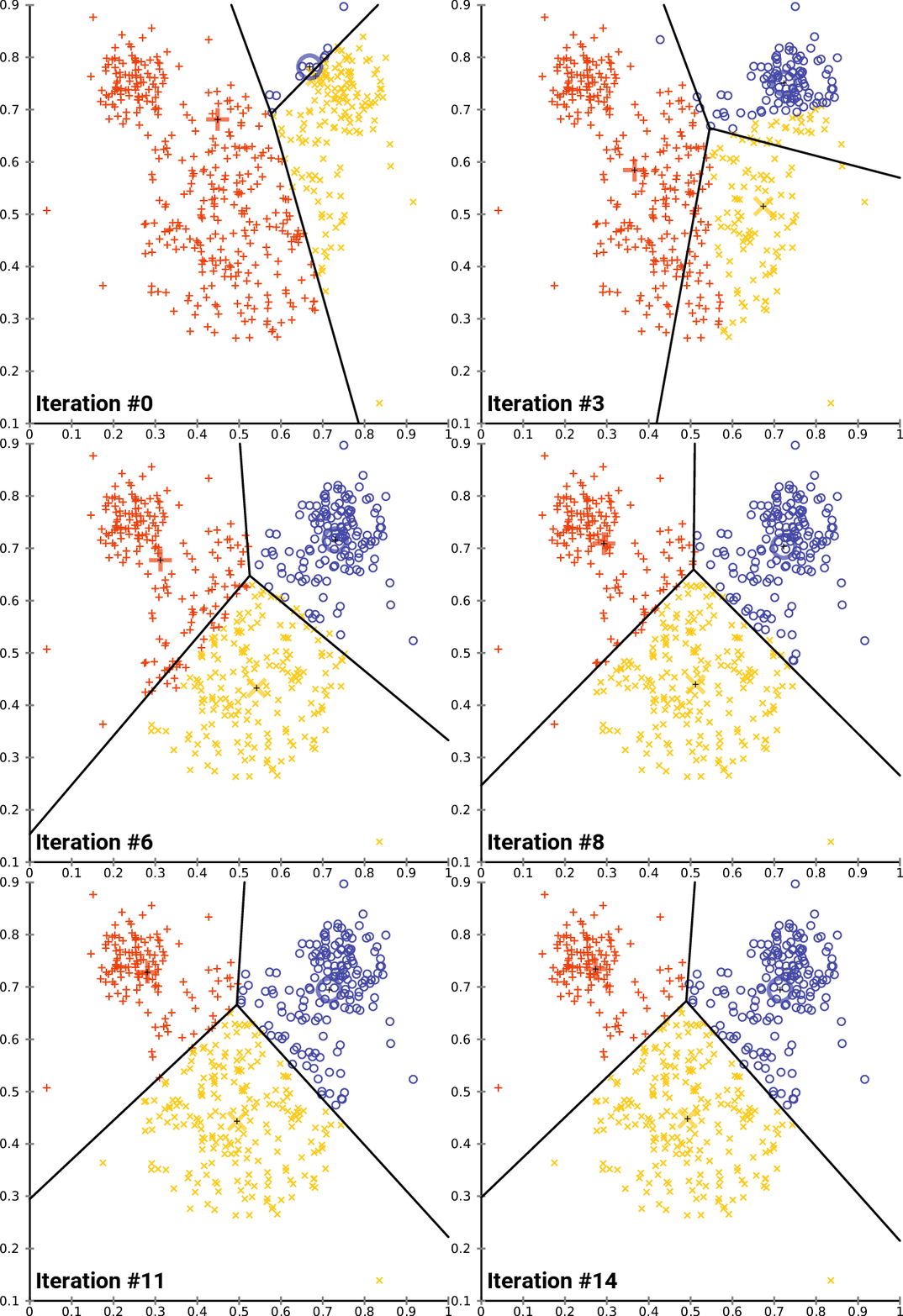
Can you see how the centroid and allocation of observations change for each iteration? It seems like the observations are getting fairly divided as the algorithm continues to be repeated.

However, there are two important points to be aware of when using the k-means algorithm. The first point is that the “starting point” is of big importance. If the starting points are somewhere isolated, then our clusters might get stuck locally as in the following illustration (source).

 

 

We can see that if we choose the wrong staring point, then the calculation of within-group distances for each cluster is stuck locally. So we have to pay close attention to where we will initialize our algorithm.

The second point is that k-means algorithm is sorely based on minimizing within-group distances, so it doesn’t consider structure of the data. Each partitioning of observations is done separately, so if we decided to use 3 clusters, then our algorithm only focuses on minimizing the within group distances for the 3 clusters. This can be problematic if our data cannot be separated based on the within group distances in the first place. An intuitive example is the following. (source)

 

 

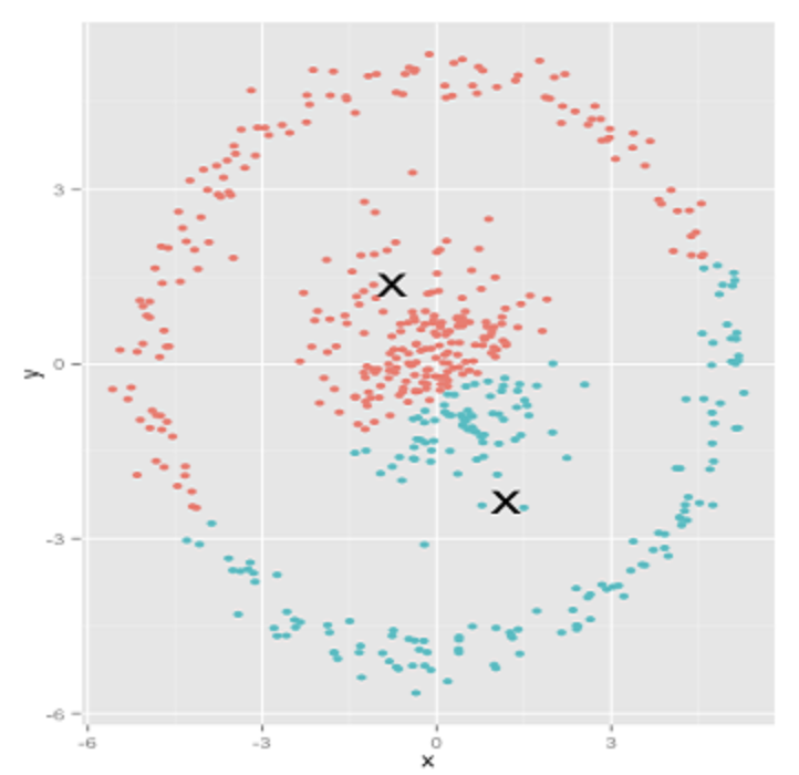
It is obvious that the clustering is done wrongly. This is the innate limitation of k-means clustering. For above data, we have to use another algorithm such as hierarchical clustering models.

Therefore, we have to always obey the working principle of our universe that there is no one-size-fits-all-approach. Although K-Means algorithm is powerful and easily implemented, always be open to different possiblities.

In practice, most of the software will automatically suggest starting points for us so our main concern would be to choose the appropriate number of clusters. There is no fixed rule for that, but keep in mind that often it is better to have smaller clusters for interpreting the results. For some practical tips on choosing the optimal number of clusters, this website provides really great tutorial so check it out if you are interested.

 

---

CA Example

Now we will perform cluster analysis to our car dataset that we’ve been using throughout this topic. We will use factoextra library in R. Full codes can be found here.

Let’s first find out the euclidean distances among the cars based on our scaled car dataset. To do that, I’ve first defined the distance matrix and created a heatmap as the following.

 

 

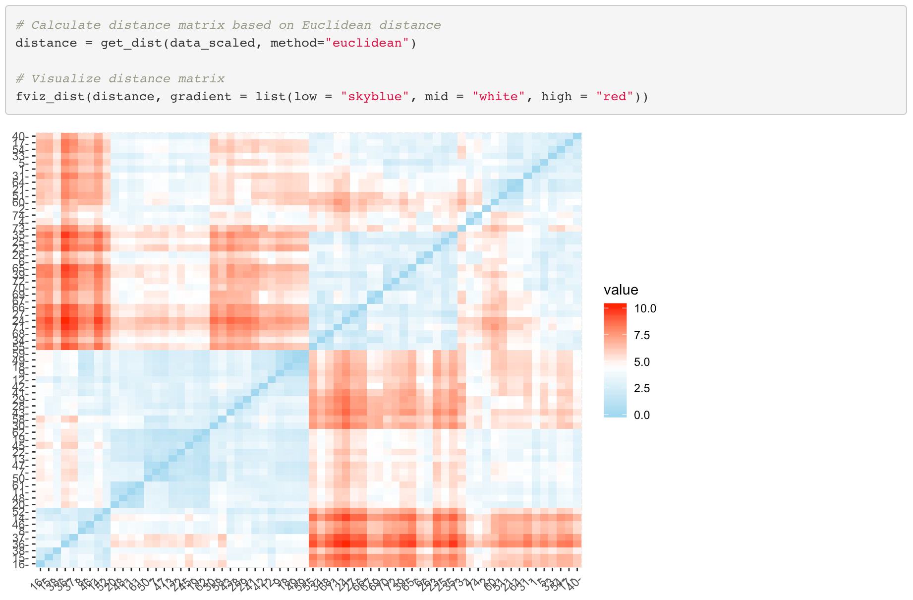
If the color is close to blue, it means that the two cars are similar and otherwise if the color is close to red. It looks like we will be able to make clusters based on the euclidean distance.

To perform cluster analysis, we first have to search for the optimal number of clusters. In our example we will use Elbow Method and Silhouette Method (Detailed introduction can be found in this website). Each methods returns a plot that can serve as a criteria to determine number of clusters to be used. Here’s the result.

 

 

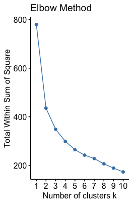
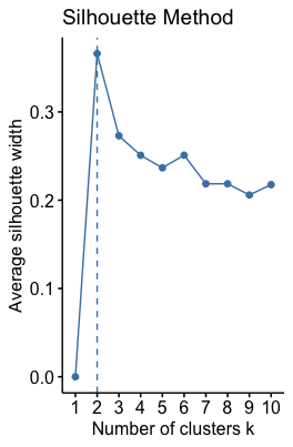
In Elbow Method we have to seek for the point where the declining slope is smoothed, just like we did in the elbow plot of PCA. On the other hand in the Silhouette Method, we want the highest point. By combining the results of two methods, it seems like 3 clusters are enough.

Based on this result, it’s time to actually implement the k-means clustering using kmeans function in R. The result is visualized on a 2-dimensional graph on the axis of the first two principal components. Each observations have color labels depending on its company values; red dot represents American cars, green dot represents Europe cars and blue dot represents Japanese cars.

 

 

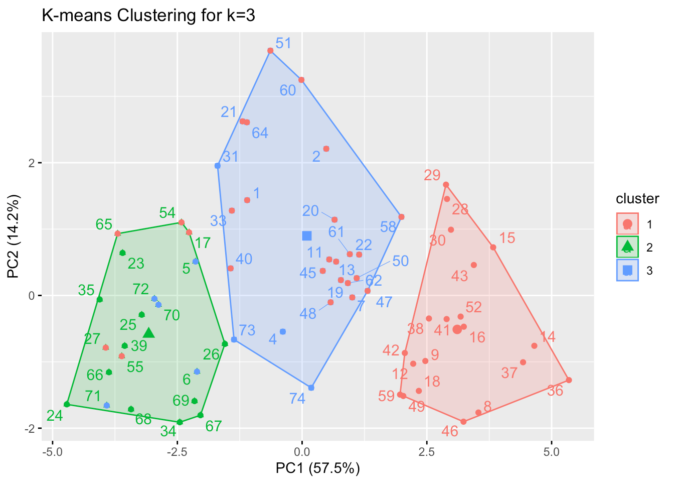
From the result, the three clusters seem to be fair enough. Note that most of the cars in the green cluster are Europe and Japanese, while the rest two clusters are mostly American cars. By this, we can infer that there is going to be some unique characteristic on Japanese and Europe cars that distinguishes them from the American cars. Moreover, there seem to be some differences within the American cars as well.

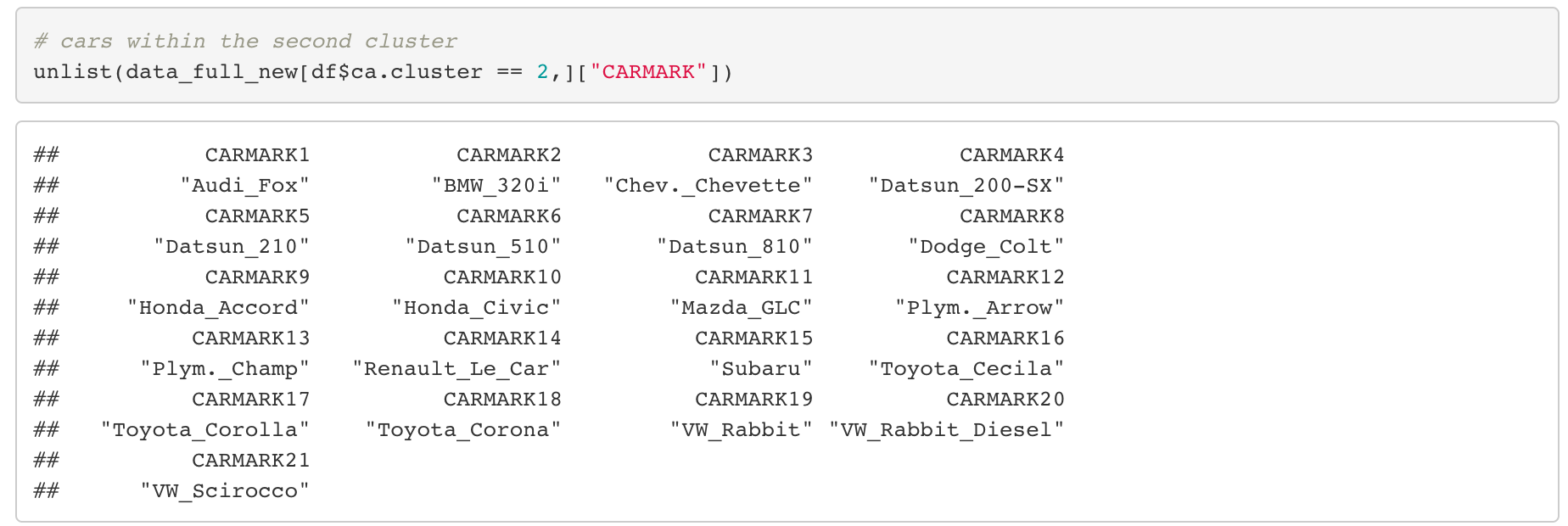
Here’s a list of car models within each clusters, so if you have sufficient knowledge on cars, it might be interesting to see if there is any trend in them.

 

Cars within the green cluster

 

Cars within the blue cluster

 

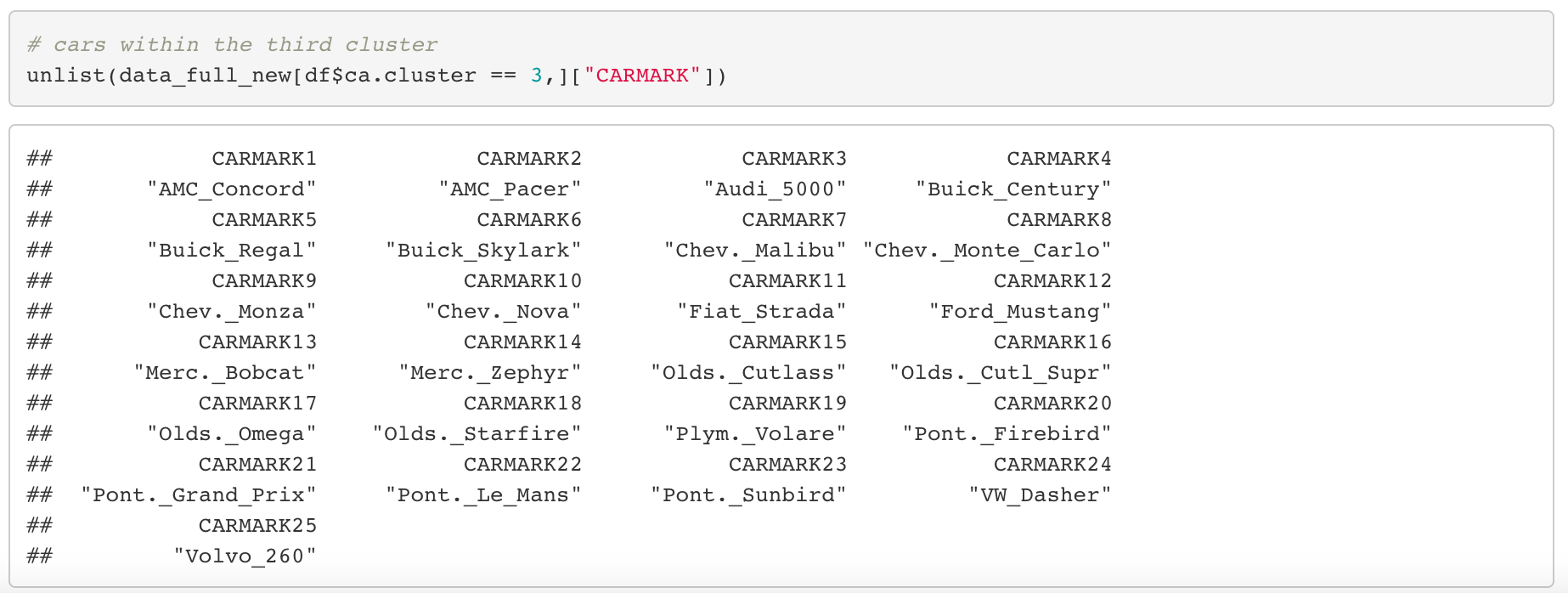
Cars within the red cluster

 

This is the end of a complete Cluster Analysis.

In the next post, we will continue talk about “Discriminant Analysis”, which is the last dimension reduction method for this topic.

---