Factor Analysis
This post will briefly introduce Factor Analysis, a statistical dimension reduction method for identifying latent variables in a dataset.
Factor Analysis (FA)
In line with PCA, Factor Analysis (FA) is another famous dimension reduction method widely used for finding latent variables. Latent variable refers to variables that are hidden. Let’s go back the example about BTS mentioned when talking about multicollinearity. The key point was that when we have variables like “width of eye”, “length of eye”, “color of eye”, these variables can be compressed into a single variable; an “eye”, which can be regarded as a latent variable hidden inside those three variables.
Often, the goal of factor analysis is to summarize the original dataset with redundant variables by extracting some hidden commonalities in them. These commonalities are called as “factors”, which are themselves insightful for subsequent statistical analysis. So it is easy to think of the factors as groups of original variables. In mathematical sense, this idea is equivalent to reducing a $p$-dimensional random vector $X$ into a fewer $k$ latent variables.
Usually most of the conventional dataset consists of continuous variables as our example will be so, but keep in mind that sometimes qualitative variables can also be used. For example, a specific dataset might include gender information, which is a nominal data that has to be encoded as [0, 1]. Even if this is the case, we can still use factor analysis to find out gender characteristics.
Then let’s dig into the details of factor analysis. By this point, one might wonder the difference between PCA and FA. This can easily be understood by looking at the equation of factor analysis.
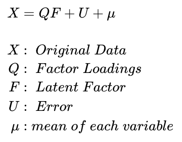
Above is the equational definition of orthogonal factor model. We can see that the original data matrix is decomposed into 3 parts. The first part is related to the unknown factors and the matrix $Q$ and $F$ are to be estimated. The second part is the error term, which accounts for individual variations in each variables. The third part is the mean of each variables, but this term is often ignored since it’s a custom to standardize each variable before analysis.
Recall that PCA was a linear transformation of X using all of the variables to create new principal components. In factor analysis, however, we decompose the original matrix into predefined factors that are limited in numbers. Since the number of factors used is smaller than the number of total variables, our factor model cannot fully retain all of the information in the original dataset as prinical component model did. Thus, some degree of noise is inevitably included. This is the main difference of PCA and FA. To put it simply, unlike PCA where we used all of the variables to re-express original dataset, FA is like a regression on the original data by a subset of variables called as factors.
Then how are we going to find matrix Q and F? The most commonly used are “Principal Component Method”, “Maximum Likelihood Method” and “Common Factor Method”, and there is no absolute criterion to ensure which one is best. Since R conveniently does that for us, we will not go detail into each methods.
The last theoritical part to look at before going into the implementation is the Factor Loadings. After performing FA, most often we will get factor loadings matrix to tell us which factor is related to which original variables. The elements of factor loadings matrix are simply the linear correlations between every factors and variables.
During the derivation of factor loadings matrix, the technic so called “Factor Rotation” is often used to maximize the relationship between factors and the original variables. What it does is that it rotates the axes of each factors at the origin until each factor loading values become close to 0 and 1 (note that each factors can be regarded as new axis similar to PCA). So basically it is sort of “exaggerating” the relationships without changing the core of data. We will see how it works in a minute, so don’t worry even if this idea is not clear at the moment.
FA example
We will use the same car data that we used for PCA. Data preprocessing is skipped as it is the same for the PCA. We will use factanal function in R. Here’s the result.
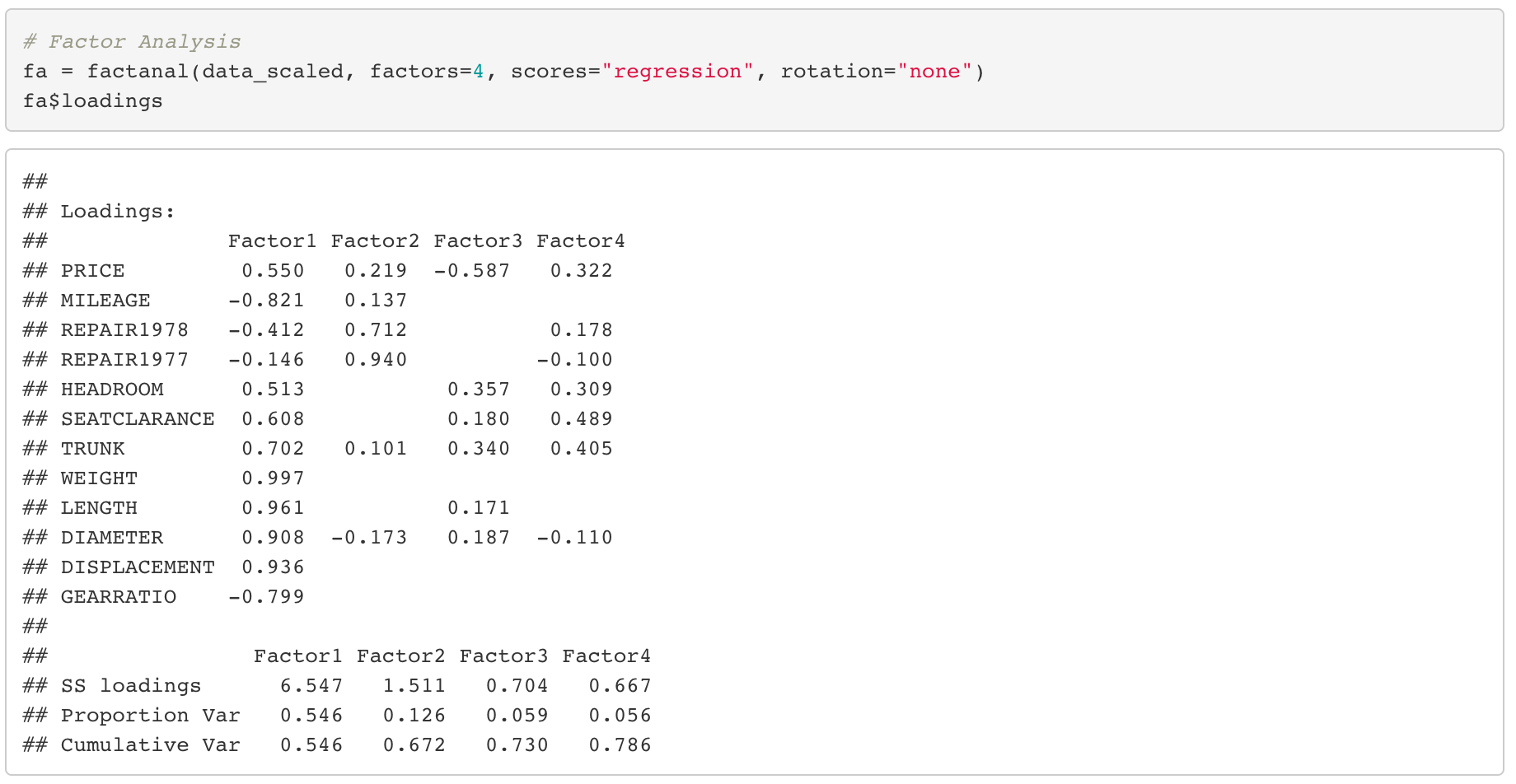
Above is factor loadings matrix for a factor analysis using 4 factors without factor rotation. The number of factors to be used is a hyper parameter that we have to choose manually and there is no rule for that.
If we use fa function in R, the following result of statistical hypothesis testing will be presented at the bottom of the result of factor analysis.

Here, the null hypothesis is “The number of factors used is sufficient”. So if the p-value is larger than the significance level, we can “statistically” say that the number of factors we have used is decent. In our example, the p-value was a little bit less than 0.05, but as having 5 factors seem too much, I would conclude to use 4 factors for our analysis.
Anyways, back to our factor loadings matrix. It seems like we have a problem. Most of the elements in the loadings matrix have values larger than 0.3. This is problematic because in this situation, we can’t really distinguish which factor is closely related to which variables. In other words, we can’t marginalize the characteristics of each factors. To deal with this problem, we are going to use factor rotation. There are various rotation methods, but among them the so called varimax rotation is mostly widely used. Let’s see what happens when we apply varimax rotation to our dataset.
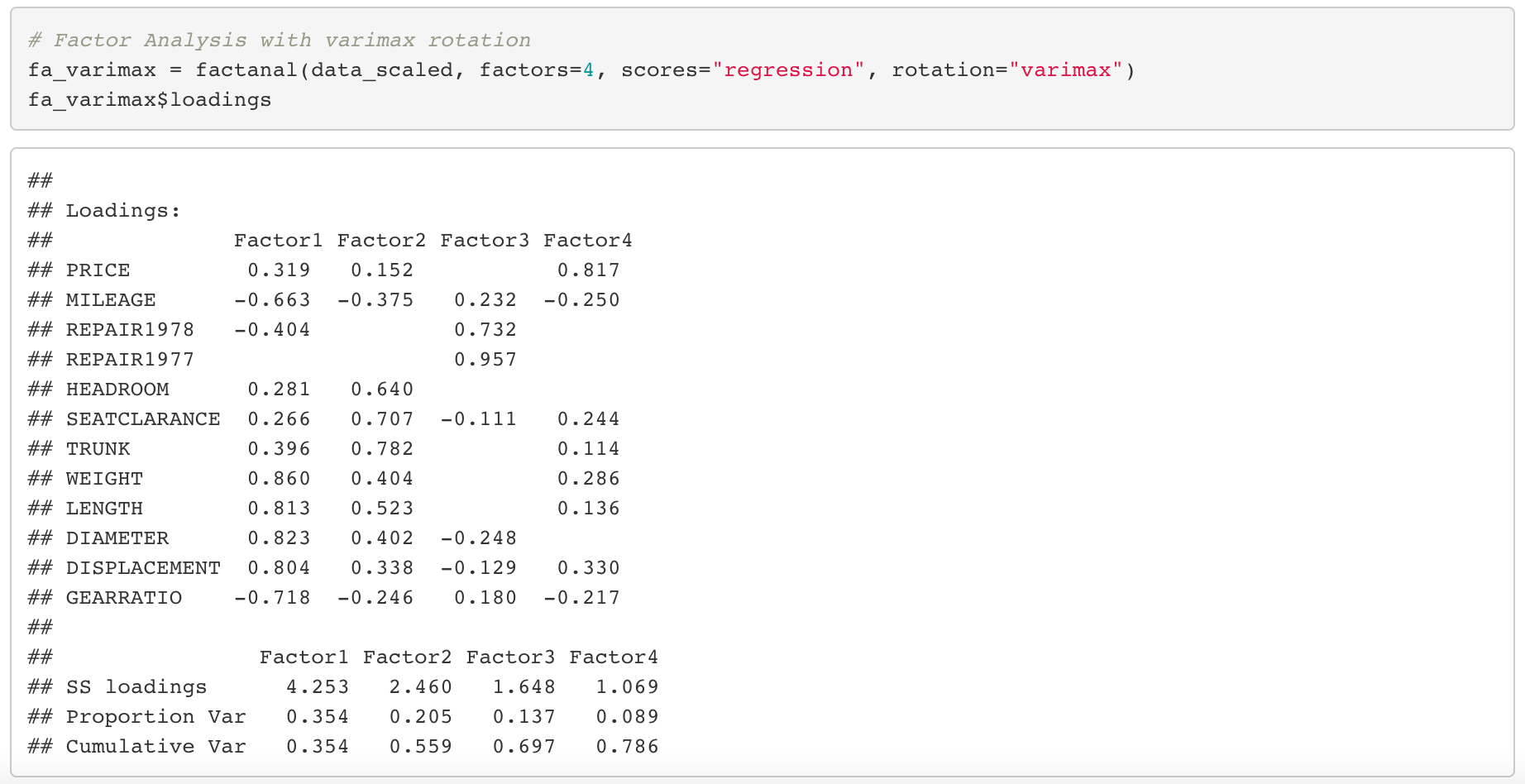
Now the values of factor loadings became relatively more clear as values are close to 0 or 1 compared to when we didn’t use rotation. Furthermore, it seems like we can name the factors. Based on the factor scores in the loadings matrix, I’ve named each factor as the following.

As always, keep in mind that interpreting the results is very subjective. Nevertheless, if we can all agree on the naming of each factors as above, it’s time to figure out if there is any pattern in the cars associated with each factors as a next step. Since we have 4 factors, it would be difficult to visualize the results in a single graph. Therefore, we will sort the car dataset by the scores of each factors. Only the result is presented here, but you can check here if you are interested in specific codes.
Factor 1 (Size of car)
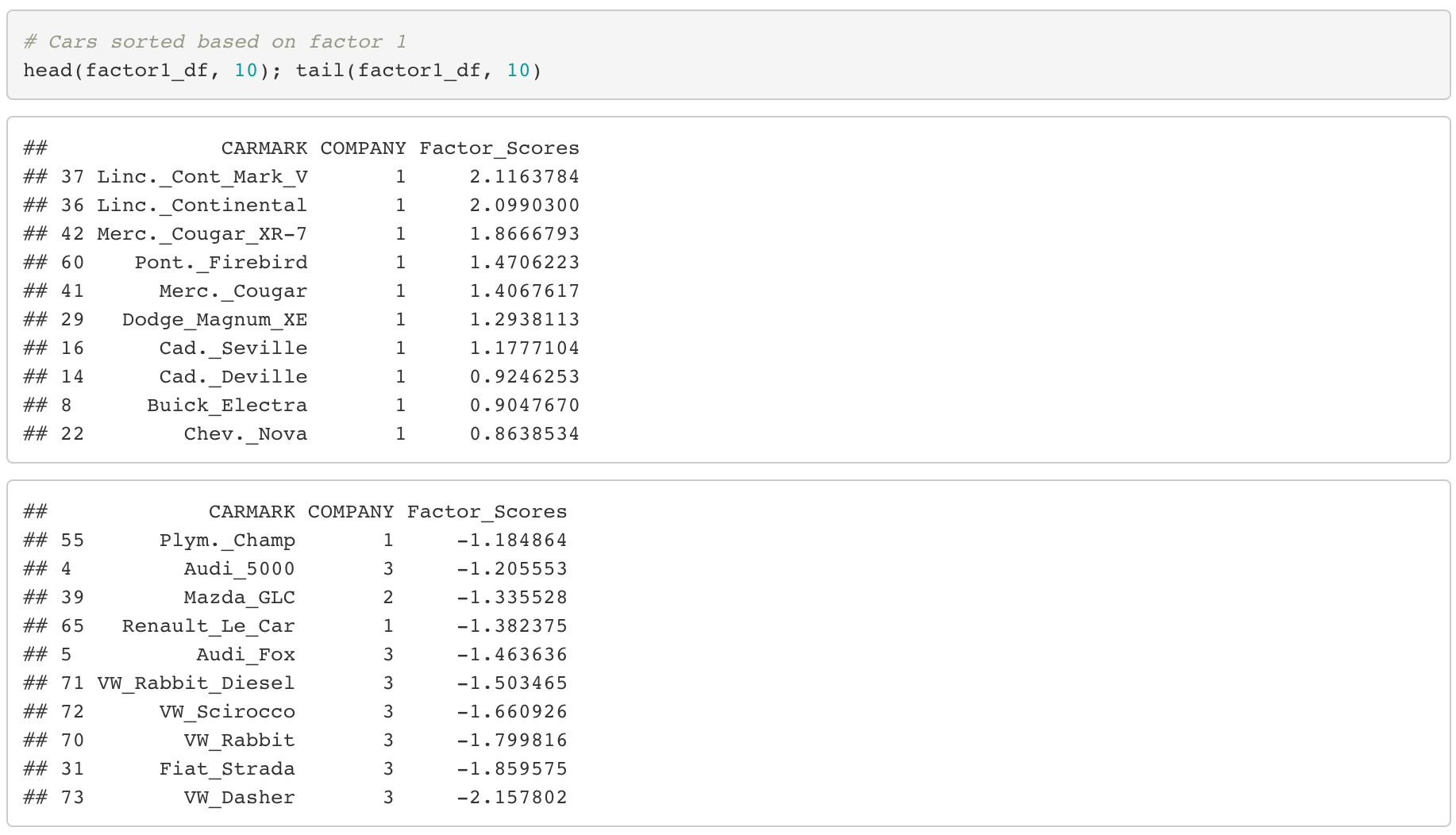
By sorting the cars according to the first factor, the top 10 cars are all from American companies as labeled “1”. On the other hand, we can see that most of cars at the bottom are European as labeled “3”.
From this, we can conclude as the following.
- In general, American cars are large in size and Europe cars are small in size.
Factor 2 (Inner space of car)
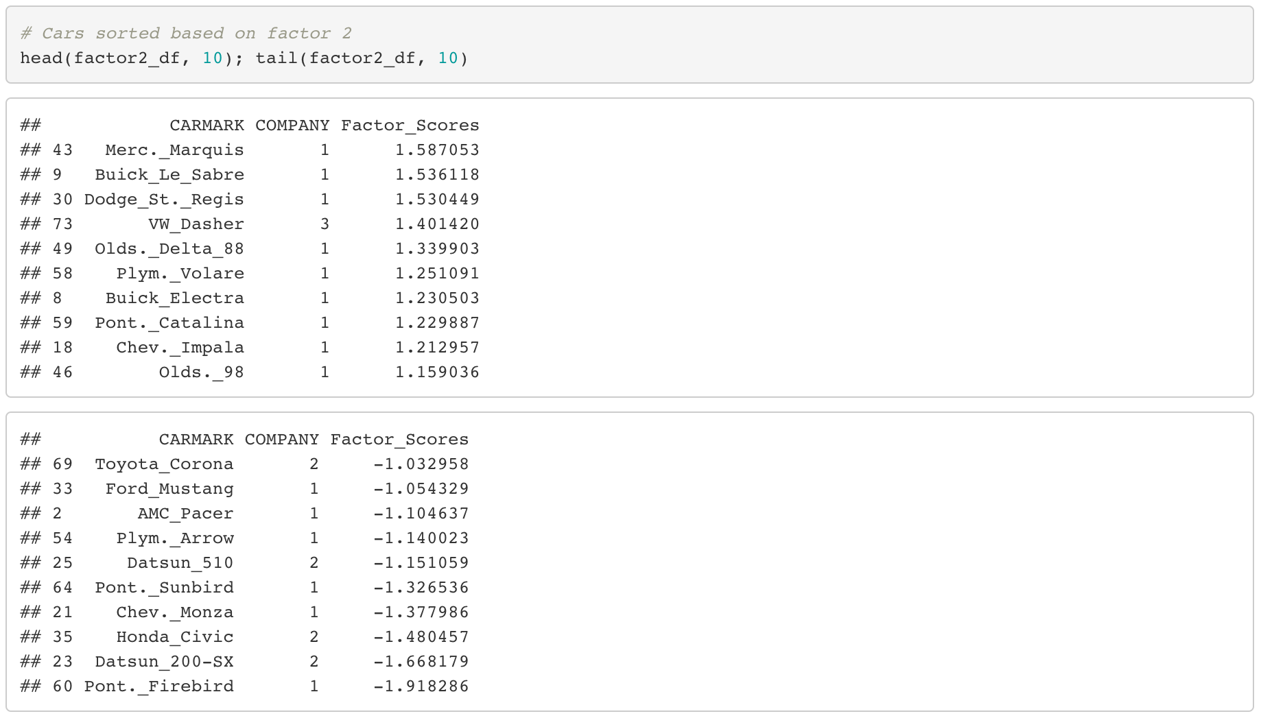
By sorting the cars in terms of the second factor, we can see that most of the cars in the top of the list are labeled as company “1”, while at the bottom relatively many cars are labeled as company “2”. This indicates the following.
- In general, American cars have larger inner spaces while japanese cars have small inner spaces.
From factor 1, we have found that American cars are usually large in size, so it’s no surprise that these cars have larger spaces inside as well.
Factor 3 (Customer Service)
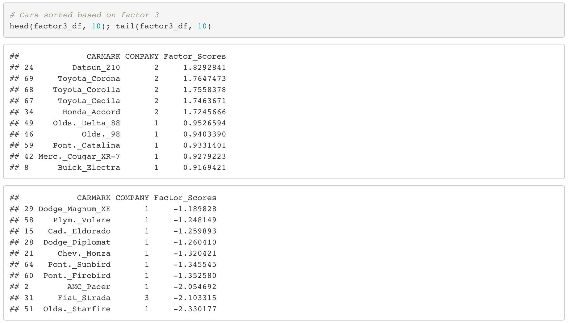
Unlike the first two factors, it is evident that the top ranked cars are all from company label “2”, meaning that they are Japanese cars.
By this, we can derive the following insight.
- Japanese cars provide good after service for customers.
Factor 4 (Price)
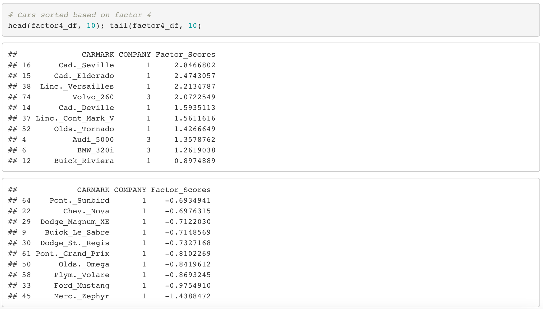
If we look at the top 10 cars, it looks like they are mostly American and European cars. But let’s focus on the models this time. They are Cadillac, Lincoln, BMW and Audi, which are high-class premium brand models. So I would say factor 4 evidently indicates price (or class) of cars.
- American cars vary a lot in terms of price, while European cars are expensive.
This is the end of a complete Factor Analysis.
For the car dataset, we were lucky that we could actually name the factors and interpret our dataset based on these findings. But in reality, there are many cases when we can’t interpret the results because factor loading scores are not distinguished clearly. So lot of rotation methods have been developed such as QUARTIMAX, EQUIMAX, VARIMAX et cetera, so check those out for a more profound and practical understanding of the Factor Analysis.
In the next post, we will move on to Cluster Analysis, which is another super cool and useful dimension reduction method.