This post will briefly introduce the concept of Linear Discriminant Analysis,

Discriminant Analysis (DA)

As a final topic of this series, we will talk about discriminant analysis and what it exactly does.

By now, all sorts of different statistical dimension reduction methods might be confusing you as they all seem to be doing similar stuffs. So before going into the details on the discriminant analysis, let’s spend some time to figure out the subtle differences in the methods we’ve studied so far.

Until now, we’ve looked at Principal Component Analysis, Factor Analysis and Cluster Analysis. Let’s focus on the main goals of each methods. First of all, CA is evidently distinctive in that it tries to group the observations by making clusters based on the distances. On the other hand, PCA, FA and DA, which is today’s topic, tries to find a linear combination of the original variables. So these later three methods are very similar by their nature, though what they aim to achieve is subtly different.

To illustrate these differences, let’s borrow some concepts from machine learning discipline. By using machine learning terms, PCA and FA are “unsupervised models” while DA is a “supervised model”. That is, unlike PCA and FA where we don’t need any output variables, Discriminant Analysis requires output classes to be supplied. This is because DA focuses on maximizing the separability between each classes. On the other hand, PCA merely aims to re-express the data in terms of components that can maximize the variance in the data, and FA tries to reveal the latent variables by focusing on the shared variance between the original variables.

To put it simply, we can summarize the differences as the following:

Hope this makes you a little less confused on the distinction between each methods.

With this in mind, it’s time to really talk about discriminant analysis. In fact, some of the details are already demonstrated. The keyword of discriminant analysis is “separation”, so we want to find some decent rule that can separate and classify the observations according to their classes. In this post we will focus on “Linear Discriminant Analysis (LDA)”, which is a major branch of DA which tries to separate observations using linear functions. However, keep in mind that in situations where our observations are intertwined strongly and thus cannot be separated by 2-Dimension lines, there’s an alternative of setting up a more complicated separation rule beyond simple lines, which is called “Quadratic Discriminant Analysis”.

Anyways, an example of discriminant analysis is “credit evaluation model”. Suppose we have data on people’s financial activities such as “number of loans”, “delinquency rate” etc, and we want to classify each people into one of the classes in between 1 ~ 10. So if a person has good traits, we want our LDA model to be able to classify that person into class 1 or 2.

To accomplish this, we must have some amount of “training dataset” with output groups specified in order to find the separation rule. These rules are obtained by using “Discriminant Function” and LDA is all about how to define and find this function.

Among the most famous rules include “Maximum Likelihood Discriminant Rule”, “Bayes Discriminant Rule” and “Fisher’s Linear Discrimination Rule”, and each methods uses different discrimination functions. However, their basic ideas are the same, which is to minimize the classification error.

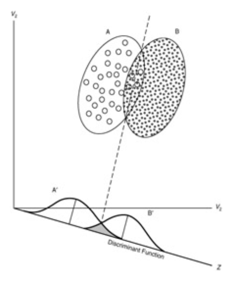
Consider above figure. The dotted line represents a linear discriminant function which serves as a milestone to separate observations into groups A and B. In the distribution function at the bottom, we see a grey zone in the middle where the two distributions are overlapped. The area of this grey zone corresponds to misclassification error. So we want a discriminant function which can minimize this area.

This is the overall concept of discriminant analysis and the various rules mentioned above are just different ways to derive this mathematically. Hence we won’t go into the details of each methods as it requires lot of formulaic deployment. Rather, we’ll see how it can be applied using a dataset. In the following example, we will use lda function in R, which by default uses maximum likelihood discriminant rule.

LDA Example

Let’s apply linear discriminant analysis to our car dataset to make a model which classifies each cars according to the company label. The detailed codes can be found on my github.

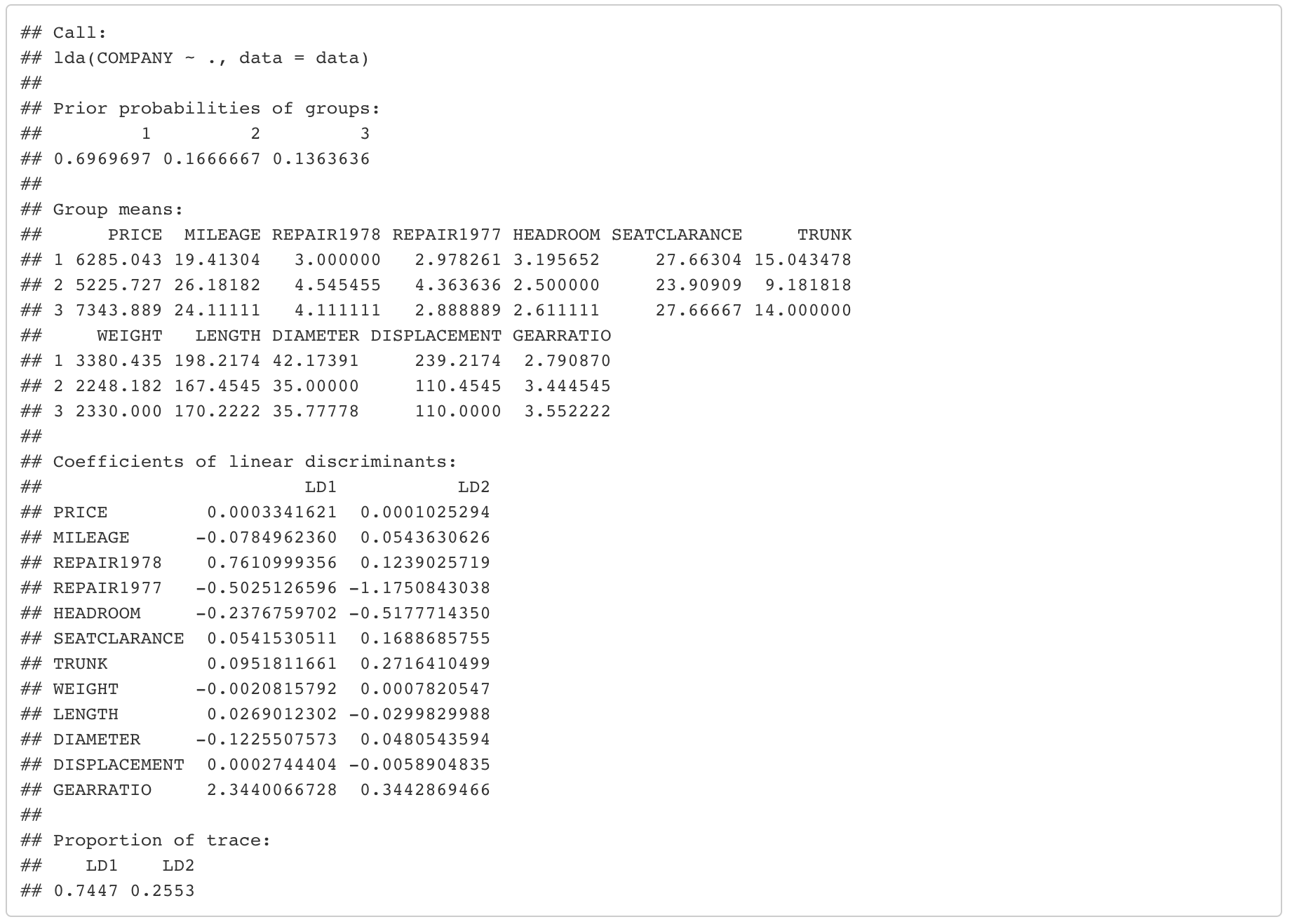
I’ve used lda function in R and the result is the following.

We can see that our model uses two discriminant functions, “LD1” and “LD2” and each of them are linear combinations of the original variable. For example, the formula of the first discriminant function, “LD1” is 0.0003*PRICE - 0.078*MILEAGE + 0.761*REPAIR1978 + ... + 0.0002*DISPLACEMENT + 2.344*GEARRATIO.

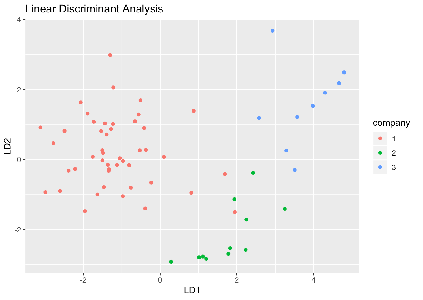
Based on these functions, individual data points of our dataset can be classified according to the company label like the following.

Although there is a little bit of overlap in company 1 and 2, it looks like we can adequately classify the cars by using linear discriminant function. If we actually calculate the missclassification rate, our model showed about 3% error, which is pretty impressive (really?).

In this example, I’ve used the entire dataset to find discriminant rule because we only had around 60 observations. However if the size of the dataset is sufficiently large, we must divide the dataset into train and test dataset with a ratio of around 80:20 in advance. This way, you can evaluate your model using the data that are not used for calculating the discriminant function and the misclassification error calculated based on this test dataset will then be an objective performance of your LDA model on a new dataset.

If we actually divide the original dataset into train/test data and run the LDA in the previous example, the misclassification error for the test dataset is the following.

We can see that the error jumped to about 14%. I think 14% is still fair enough, so we can stick to our original judgement that LDA seems to fit well to our car dataset.

As a last reminder, using fancy model doesn’t guarentee good performance. Even if we used quadratic discriminant analysis in the cars dataset, there is no guarentee that the misclassification error on the test dataset will be reduced. This is because our model tries to find a discriminant rule which best suits our train dataset, not test dataset, and this issue is formally called as Overfitting. This is a very sensitive issue in machine learning models and cross validation technics are often applied to measure the true performance of a trained model.