[Bayesian Statistics] Metropolis-Hastings

2021, Feb 21

 

This post briefly explains the Metropolis-Hastings algorithm, which is a algorithmic methodology of MCMC in a Bayesian posterior inference.

 

Previous Posts

1. Bayesian Statistics - Basics

2. Bayesian Statistics - Conjugacy

3. Bayesian Statistics - Hierarchical Models and Monte Carlo Simulation

 

---

When and why do we need MCMC?

In the previous post, we saw that we cannot derive the posterior analytically when we have the following setup of prior and likelihood.

 

$$ likelihood:\;\;\;\;y_i | \mu,\sigma^2 \stackrel{iid}{\sim} N(\mu, \sigma^2)\\ prior\;of\;\mu: \;\;\;\; \mu|\sigma^2 \sim N(\mu_0, \frac{\sigma^2}{w_0}) \\ prior\;of\;\sigma: \;\;\;\;\ \sigma^2 \sim IG(\nu_0, \beta_0) $$

 

Although we know we can’t, let’s try it out to examine where exactly we get stuck.

 

$$ \begin{aligned} f(\mu, \sigma^2 | y_1,...,y_n) &\propto f(y_1,...,y_n|\mu,\sigma^2)f(\mu|\sigma^2)f(\sigma^2) \\[10pt] &= \prod_{i=1}^n\{N(y_i|\mu,\sigma^2)\} \; N(\mu|\mu_0, \frac{\sigma^2}{w_0}) \; IG(\sigma^2|\nu_0, \beta_0) \\[10pt] &= \prod_{i=1}^n\{\frac{1}{\sqrt{2\pi\sigma^2}}exp(-\frac{1}{2\sigma^2}(y_i-\mu)^2)\} \{\frac{1}{\sqrt{2\pi\sigma_0^2}}exp(-\frac{1}{2\sigma_0^2}(\mu-\mu_0)^2)\} \{\frac{\beta_0^{\nu_0}}{\Gamma(\nu_0)}(\sigma^2)^{-(v_0+1)}exp(-\frac{\beta_0}{\sigma^2})\} \\[10pt] &\propto \{(\sigma^2)^{-\frac{n}{2}}exp(-\frac{1}{2\sigma^2}\sum_{i=1}^n(y_i-\mu)^2)\} \{exp(-\frac{1}{2\sigma_0^2}(\mu-\mu_0)^2)\} \{(\sigma^2)^{-(v_0+1)}exp(-\frac{\beta_0}{\sigma^2})\} \end{aligned} $$

 

From the last part of the equation, we have a very complicated form of the posterior kernel even after we have removed all the terms that are independent of $\mu$ and $\sigma^2$. Thus, we cannot not go further and we have to conclude that the posterior cannot be derived as a close-form.

On the other hand, even under the circumstances, we can use Monte-Carlo simulation and approximate our sample distribution to the posterior like I introduced in the previous post. This methodology is called as MCMC and let’s now see how it works.

 

---

Principle of MCMC

As its name implies, MCMC is an abbreviation that stands for Markov Chain - Monte Carlo. In short, it is a collection of efficient sampling methodologies which is based on the mathematical concepts of Markov Chain and Monte Carlo. With that being said, let’s see how the two components are used in the MCMC.

From a given probability distribution, MCMC draws random samples based on the previously generated sample. In other words, only the current state is involved in the process of generating the next state, which is a characteristic of Markov Chain. In theory, Markov Chain has a stationary distribution if it satisfies what is known as Detailed Balance Condition. Roughly speaking, stationary distribution is the limiting distribution of a specific Markov Chain. For example, if we infinitely repeat rolling a six sided fair dice, then the probability of each eyes will converge to the stationary distribution of $p(x_i) = \frac{1}{6}, \;\;(i = 1, … , 6)$.

Using this principle of Markov Chain, MCMC defines a Markov Chain whose stationary distribution is the target distribution of our interest. Then our Markov Chain moves around the parameter space to collect random samples and based on these samples we can apply Monte-Carlo methods to get the posterior distribution like we did in the previous post.

In summary, we are using MCMC to approximate the posterior distribution from a well-defined Markov Chain by moving around the states and getting samples to apply the Monte-Carlo method. Thus, the success or failure of a MCMC critically depends on the quality of the samples, which is determined by how effieciently the Markov Chain can explore our parameter space. There are various MCMC algorithms and for now, we will focus on the most basic and fundamental sampling method known as Metropolis-Hastings algorithm.

 

---

Metropolis-Hastings Algorithm

Metropolis-Hastings is a MCMC method for collecting a sequence of random samples from a probability distribution where direct sampling is difficult. Suppose we are interested in evaluating the following posterior distribution.

 

$$ f(\mu | y_1,...,y_n) \propto \frac{exp\{n(\bar y\mu - \frac{\mu^2}{2})\}}{1+\mu^2} $$

 

Because of the normalizing constant $1+\mu^2$ of the denominator, we cannot define the posterior as a closed-form probability distribution. Considering this example, let’s use Metropolis Hastings algorithm to evaluate the posterior.

 

---

<Steps of MH>

 

(1)

Define a function $g(\mu)$ that is proportional to our target distribution $f(\mu)$.

 

(2)

Furthermore, define a conditional probability distribution \(q(\mu' | \mu)\) , which is easy to get samples from. In general, standard distributions like normal distribution is used. This distribution is called as proposal distribution.

 

(3)

Since we don’t know the transition probability of our Markov Chain, randomly draw a candidate $\mu_{t+1}$ from the proposal distribution and decide whether to accept the candidate as our next sample or not by comparing the difference between \(q(\mu_{t+1} | \mu_t)\) and \(f(\mu_{t+1} | \mu_t)\) by acceptance ratio $\alpha_{t, t+1}$.

 

(4)

In rejection sampling scheme, we define an acceptance ratio which is a probability to accept the proposed state $\mu_{t+1}$. (I will not go into the details of rejection sampling here, but note that Metropolis Hastings algorithm is an application of rejection sampling)

$$ \alpha_{t, t+1} = \frac{f(\mu_{t+1}|\mu_t)}{q(\mu_{t+1}|\mu_t)} $$

This ratio being equal to 1 means that we accept the candidate because the sample is just as likely to have came from the proposal distribution as the target distribution (Note that in rejection sampling, $q$ is an upper bound of our target distribution so the acceptance ratio cannot be greater than 1).

$$ f(\mu_{t+1} | \mu_t) = q(\mu_{t+1} | \mu_t) $$

However, for most of the time it will be vice versa, that the acceptance ratio will be less than 1. In this case we are not sure about our candidate sample, so we “probabilistically” accept our candidate to be the next sample.

 

(5)

Likewise, we need to define an acceptance ratio for our Metropolis Hastings algorithm in a way that our Markov Chain satisfies the Detailed Balance Condition.

$$ detailed\;balance\;condition: \;\;\;\; \frac{f(x|x')}{f(x'|x)} = \frac{f(x)}{f(x')} $$

 

The transition probabilty can be represented as following.

$$ \begin{aligned} f(\mu_{t+1}|\mu_t) &= q(\mu_{t+1}|\mu_t) \alpha_{t,t+1} \\[10pt] f(\mu_t|\mu_{t+1}) &= q(\mu_t | \mu_{t+1})\alpha_{t+1, t} \end{aligned} $$

 

Plug this equation to the detailed balance condition and we get

$$ \frac{f(\mu_t)}{f(\mu_{t+1})} = \frac{q(\mu_t | \mu_{t+1})\;\alpha_{t+1, t}}{q(\mu_{t+1}|\mu_t)\;\alpha_{t,t+1}} \\[20pt] \Leftrightarrow \\[10pt] \begin{aligned} \frac{\alpha_{t,t+1}}{\alpha_{t+1,t}} &= \frac{f(\mu_{t+1})q(\mu_{t}|\mu_{t+1})}{f(\mu_t)q(\mu_{t+1}|\mu_{t})}\\[10pt] &= \frac{g(\mu_{t+1})q(\mu_{t}|\mu_{t+1})}{g(\mu_t)q(\mu_{t+1}|\mu_{t})} \end{aligned} $$

 

Thus if we define acceptance ratio \(\alpha_{t, t+1} = min(1, \frac{g(\mu_{t+1})}{g(\mu_t)}\frac{q(\mu_t|\mu_{t+1})}{q(\mu_{t+1}|\mu_t)})\) , then it satisfies the detailed balance condition because either $\alpha_{t, t+1}$ or $\alpha_{t+1, t}$ is always 1.

Note that if we use symmetric proposal distribution, the calculation gets much simpler because \(q(\mu_t | \mu_{t+1}) = q(\mu_{t+1}|\mu_t)\) . In fact, this is the Metropolis algorithm, and Metropolis Hastings can be seen as a extension of Metropolis algorithm.

 

(6)

Repeat above steps until our Markov Chain converges.

---

Above is a specific step-by-step illustration of the algorithm, but for practical implementation these steps can be simplified as the following.

 

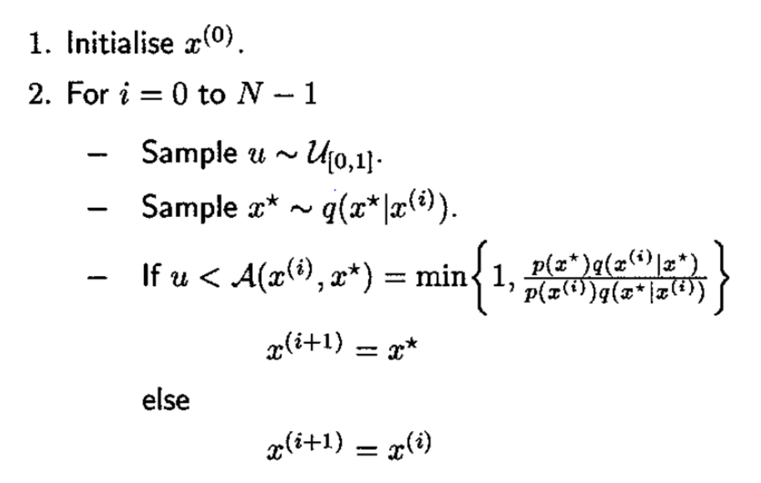
Simplification of MH Algorithm for implementation

 

Now it’s time to actually implement Metropolis Hastings algorithm using Python!

 

---

Metropolis-Hastings in Python

Normally, we wouldn’t have to bothered about implementing these MCMC algorithms because we can just use the built-in functions from the module pymc3 or jags, which provides us with a high-level abstraction. But for the sake of learning, we will hard-code MH algorithm and see how it works.

Here’s the setting of our problem that we would like to derive the posterior from.

 

$$ \begin{aligned} likelihood:\;y_i|\mu \stackrel{iid}{\sim} N(\mu, 1)\\[10pt] prior:\;\mu \sim t(0,1,1)\\[10pt] \end{aligned} $$   $$ \begin{aligned} f(\mu|y_1,...y_n) &= \frac{f(y_1,...y_n|\mu)f(\mu)}{\int f(y_1,...y_n|\mu)f(\mu)du}\\[10pt] &\propto f(y_1,...,y_n)f(\mu)\\[10pt] &= \prod_{i=1}^n [N(y_i|\mu)] [t(\mu|0,1,1)]\\[10pt] &= \frac{1}{\sqrt{2\pi}}exp(-\frac{1}{2}\sum_{i=1}^n (y_i-\mu)^2)\frac{1}{1+\mu^2}\\[10pt] &\propto \frac{exp(n(\bar{y}\mu - \frac{\mu^2}{2} ))}{1+\mu^2} \end{aligned} $$

 

In this setting, we are interested in finding out the distribution of $\frac{exp(n(\bar{y}\mu - \frac{\mu^2}{2} ))}{1+\mu^2}$ that has no closed-form solution. For simplicity we will use the symmeric proposal distribution, so strictly speaking, we are implementing Metropolis algorithm which is a special case of Metropolis Hastings.

---

1. Define $g(\mu)$

We define $g(\mu)$ to be the log-scaled version of the original function to prevent possible underflow errors.

 

2. Random Walk Metropolis algorithm

 

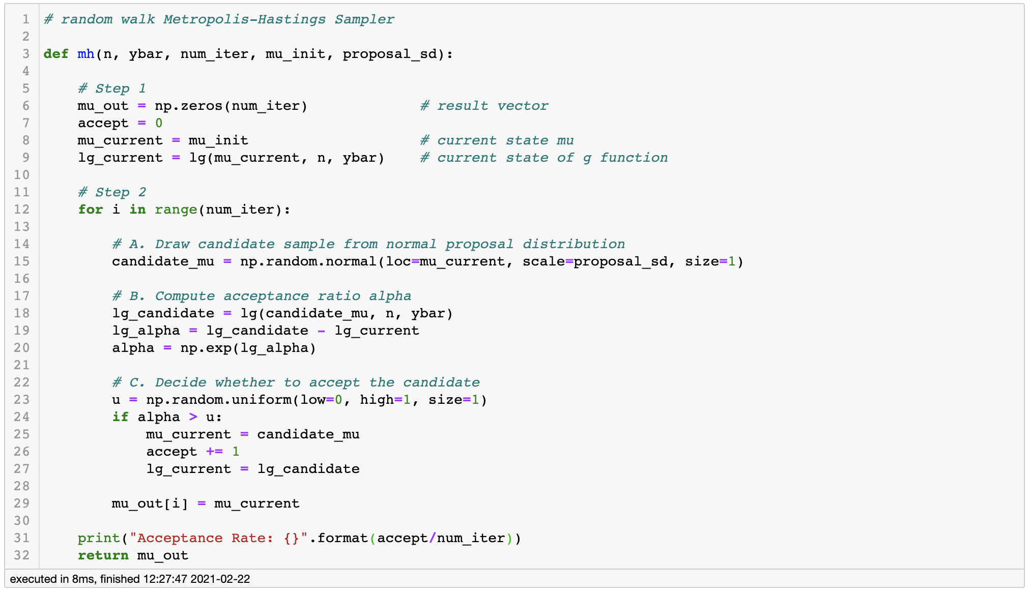
3. Apply Metropolis algorithm - Bad Example

Let’s suppose that we have 9 observations such that [1.2, 1.4, -0.5, 0.9, 2.3, 1.0, 0.1, 1.3, 1.9].

 

Using these observations, let’s sample 1,000 posterior samples. The choice of hyperparameter of the proposal distribution effects the speed of the convergence, so it is important to use descent starting point. First, let’s set the standard deviation of our proposal distribution to be 5 and see what happens.

There are several ways of examining the quality of our MCMC samples, and here we will use trace plot.

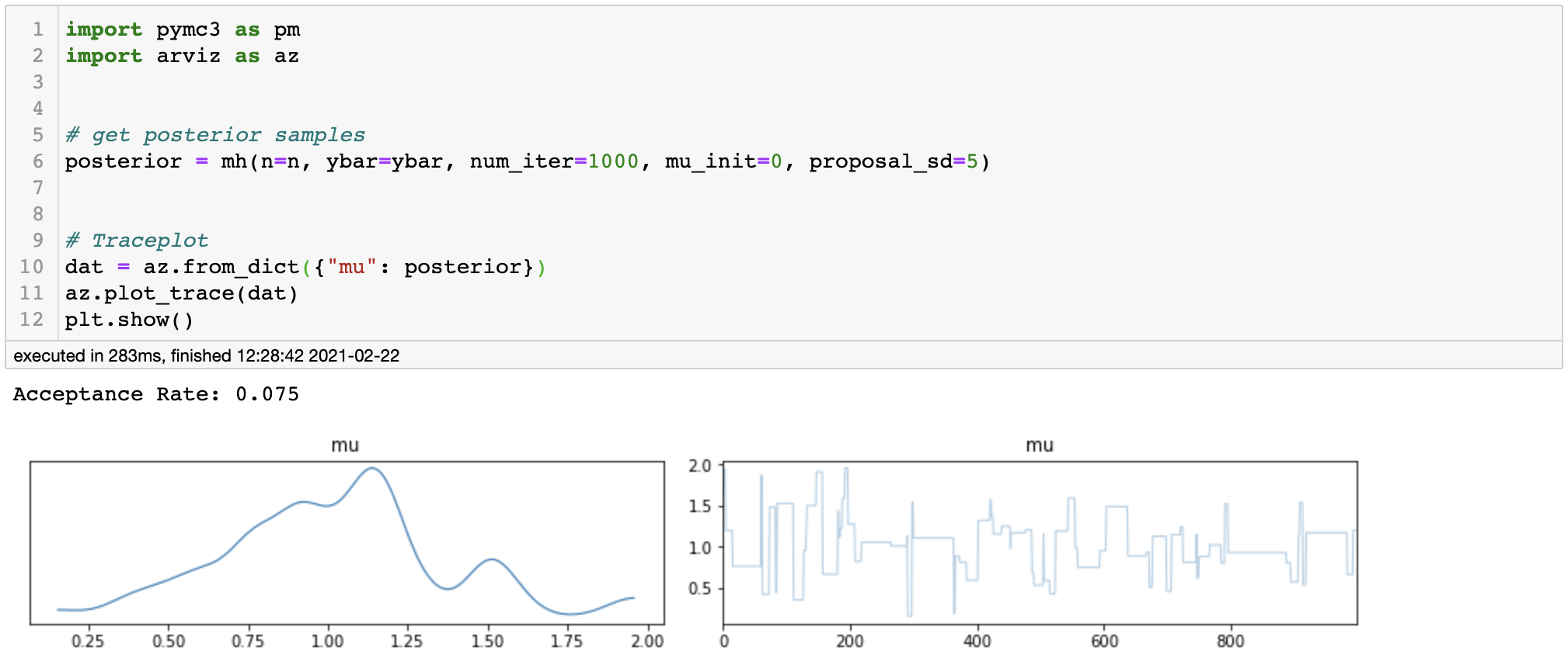
posterior kde and trace plot for high variance

 

If we look at the trace plot, we can see that our Markov Chain is frequently stucked in some states during the iterations. Our acceptance rate is only about 0.075, meaning that the samples were frequently rejected because the variance was set too big. Ideally, we would want our acceptance rate to be within 0.23 ~ 0.5.

On the other hand, let’s see what happens if we use too small standard deviation for the proposal distribution.

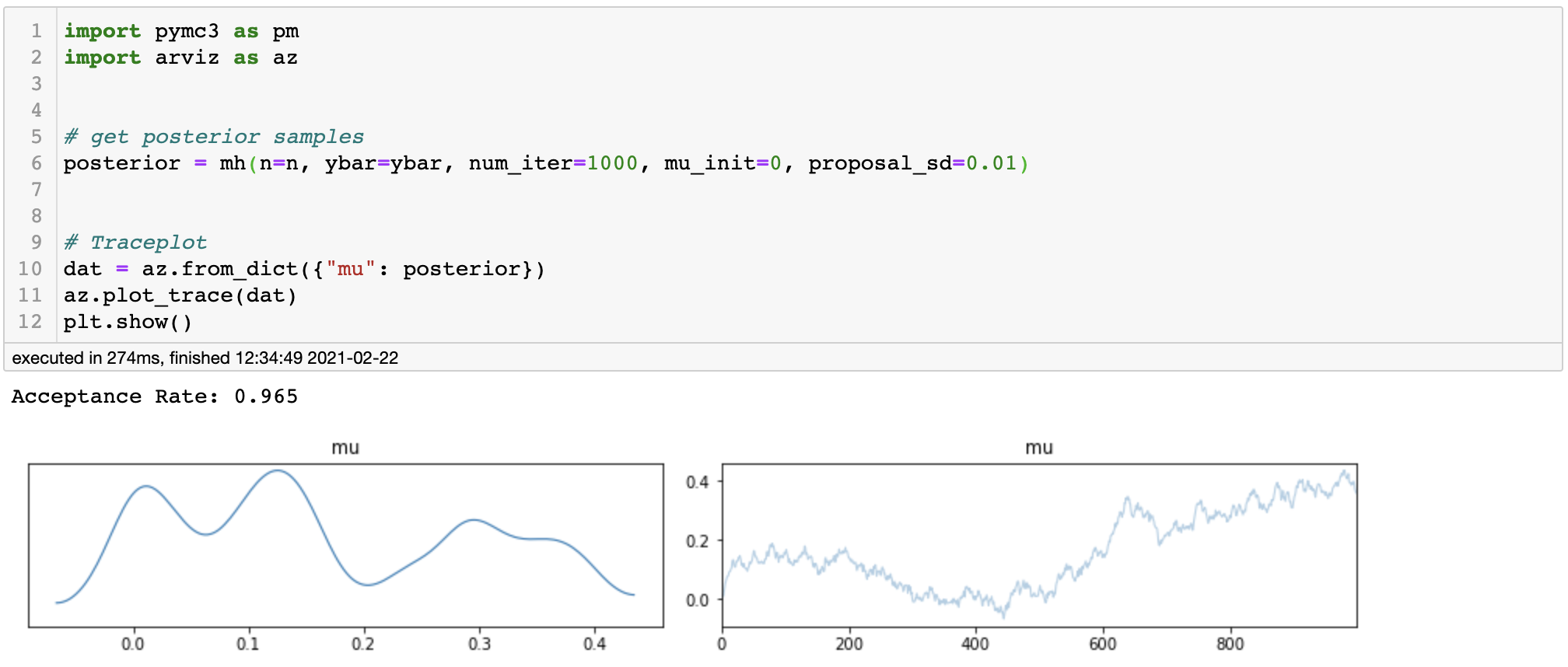
posterior kde and trace plot for small variance

 

We can clearly find an upward-moving pattern in the trace plot and the acceptance rate is as high as 0.965. This indicates that our Markov Chain has unduly accepted the candidates, resulting in a highly correlated posterior samples which are practically of no importance.

There are two remedies to this problem - first is to find ideal starting point, and second is to increase the number of iterations.

 

4. Apply Metropolis algorithm - Good Example

This time, we will use standard normal distribution as our proposal distribution, which is assumed to perform well under our metropolis algorithm.

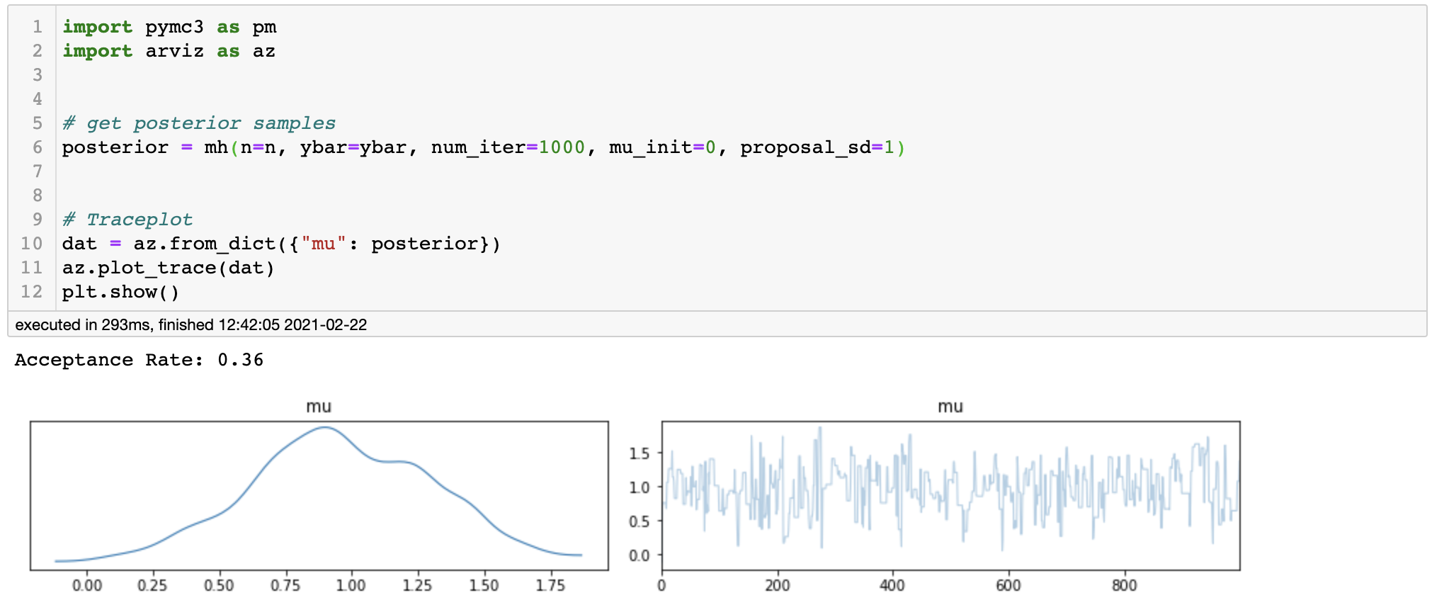
posterior kde and trace plot for optimal variance

 

We can see that our trace plot randomly moves around the mean without any patterns and the acceptance rate is about 0.36, which altogether is good. Thus, we can conclude that our Markov Chain seem to have converged to the stationary distribution (which in this case is the posterior distribution).

 

5. Posterior Analysis

Now let’s try visualize the result of our MCMC simulation.

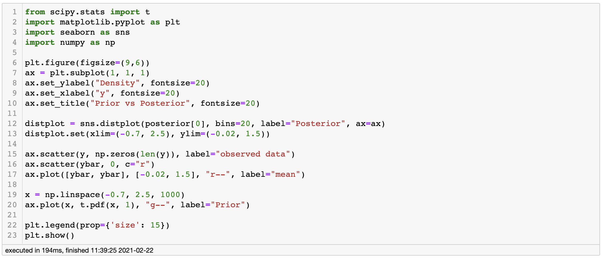
By running this code we get the following plot.

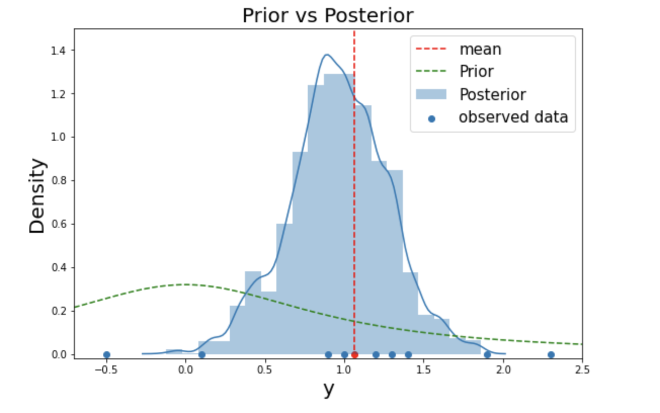
Fig. 1. Comparision of the posterior with the prior

 

We can see that the prior has moved to the center of the observations and formed a posterior, which matches our intuition. This is indeed a satisfactory result and we managed to derive the posterior of $\frac{exp(n(\bar{y}\mu - \frac{\mu^2}{2} ))}{1+\mu^2}$, which we couldn’t analytically.

We have successfully derived the posterior using Metropolis-Hastings sampler! However, this method has some limitations as MH sampler gets very inefficient when we are dealing with posteriors that have multiple parameters. In the following post, we are going to take a look at another MCMC method - Gibbs Sampler, which is designed to work well on the multi-parameter problems as well.

---

 

Remarks

There are some important points worth paying attention when making inference about the posterior using MCMC.

First, regarding the convergence of the Markov Chain, our Markov Chain is guarenteed to converge to the stationary distribution using MCMC methods if we have infinitely many samples. However it is just in theory and we can’t afford to sample infinitely. Therefore, we have to endure some possible tradeoff between the accuracy and computational practicality. In practice, we use several parallel Markov Chains with different starting points to assure that the chains converge to the same stationary distribution.

Second, we should only use the samples that are simulated after the Markov Chain has converged. In other words, we have to exclude the primal samples of the chains for making inferences. The time until the convergence is called as the burn-in period.

Third, posterior samples are inevitably dependent with each other as they have been simulated from a Markov Chain. Therefore it is important to check the effective sample size for the posterior samples, which indicates the amount of independent information in them.

Fourth, assessment of the quality of the posterior samples can be done in a various ways where trace plot is the most simple and straightforward method. Apart from the trace plot, we can also numerically diagnose the convergence of our Markov Chain by using r-hat (or Gelman-Rubin convergence diagnostics).

Fifth, different samplers have different performances. This is a big problem as we are interested in a high-dimensional, multi-modal posterior distributions where simple Metropolis-Hastings Sampler does not work. We will talk more about this in the future, but for now be aware that Metropolis-Hastings is a very basic MCMC algorithm. In practice we use more complicated MCMC algorithms such as NUTS (No U-Turn Sampler) and HMC (Hamiltonian Monte-Carlo). In fact NUTS is the default sampler of pymc3 module.

---

 

References

• Gelman et. al. 2013. Bayesian Data Analysis. 3rd ed. CRC Press.
• Wikipedia-Metropolis Hastings