[Bayesian Statistics] Gibbs Sampling
This post is a gentle introduction to the Gibbs Sampling algorithm which is a MCMC method designed for high dimensional posteriors.
Previous Posts
1. Bayesian Statistics - Basics
2. Bayesian Statistics - Conjugacy
3. Bayesian Statistics - Hierarchical Models and Monte Carlo Simulation
4. Bayesian Statistics - Metropolis-Hastings
Shortcomings of Metropolis-Hastings
In the previous post we have implemented Metropolis-Hastings sampler on the following example.
We assumed that the parameter $\sigma^2$ was given for the prior predictive normal distribution because Metropolis-Hastings algorithm is designed to work well on the single-parameter unimodal distributions. In fact, its performance tends to get poorer for multi-parameter and multimodal problems.
For example, take a look at the following simulation of Metropolis-Hastings sampling process from a bivariate-trimodal posterior distribution. The code for the simulation is written by Chi Feng.
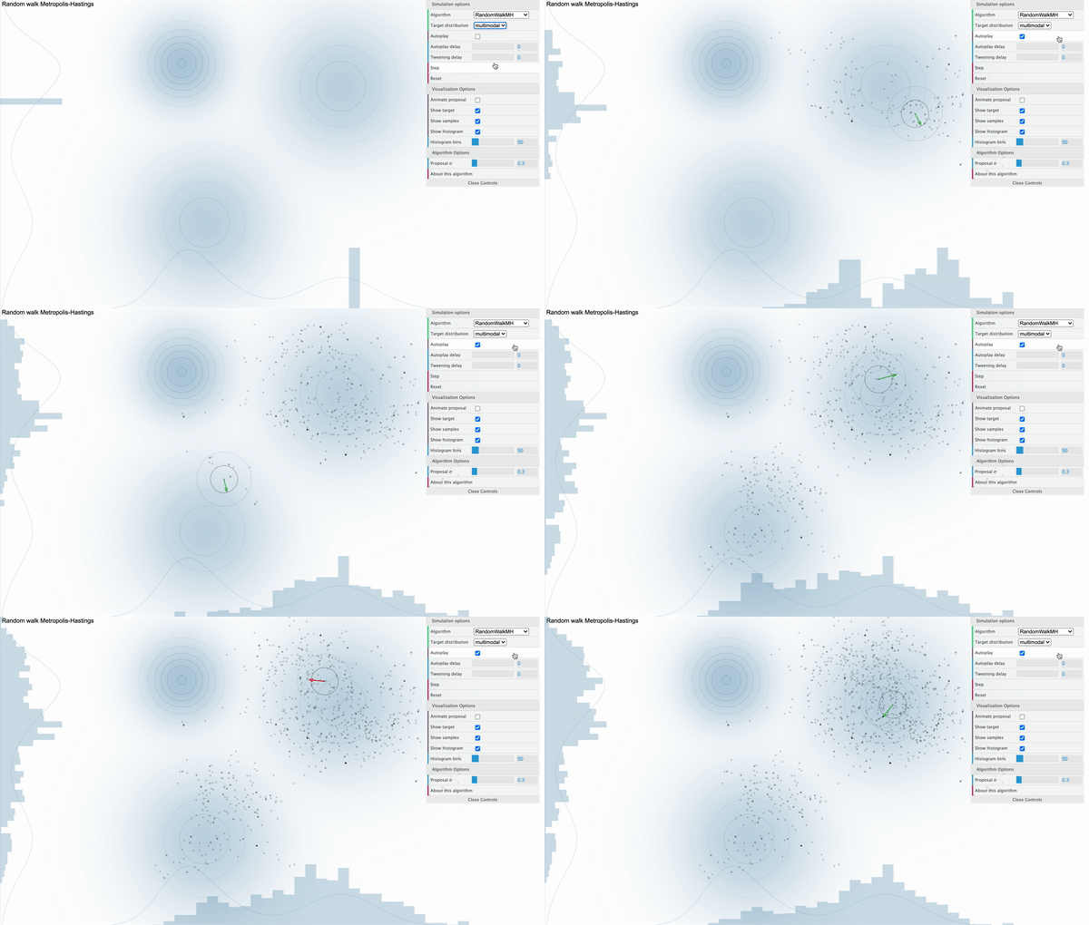
Metropolis-Hastings with Normal proposal distribution with sd 0.3
We can see that our sampler cannot explore the parameter space efficiently as it tends to get stuck in the local mode. This is because the way how sampling is done strongly depends on the parameterization of the proposal distribution. That is, if we use proposal distribution with low variance, our Markov Chain cannot take big steps enough to move between different modes. Furthermore, the calculation of conditional distribution of the proposal distribution in the acceptance ratio gets complicated as we have more parameters, decreasing the speed of convergence.
As a possible remedy for this problem, we are going to take a look at another famous MCMC method, Gibbs Sampler, which is known to be working well with multi-parameter distributions.
What is Gibbs Sampling?
To account for realistic data of our world, we will most likely be using complicated models with multiple parameters. It is needless to say that we cannot derive the posteriors analytically in these models as most of them are not defined in a closed-form distribution.
To handle this problem Gibbs sampler starts with the idea that if considering all of the parameters at once is difficult, then we can just deal with them one at a time sequentially. Formally speaking, the main idea of Gibbs Sampling is to reduce multidimensional sampling to a sequence of 1-dimensional samplings, which can be regarded as a kind of dimension reduction.
Before digging into the details of Gibbs Sampling method, let’s take a look at how it performs on the above posterior distribution which Metropolis-Hastings had trouble with.
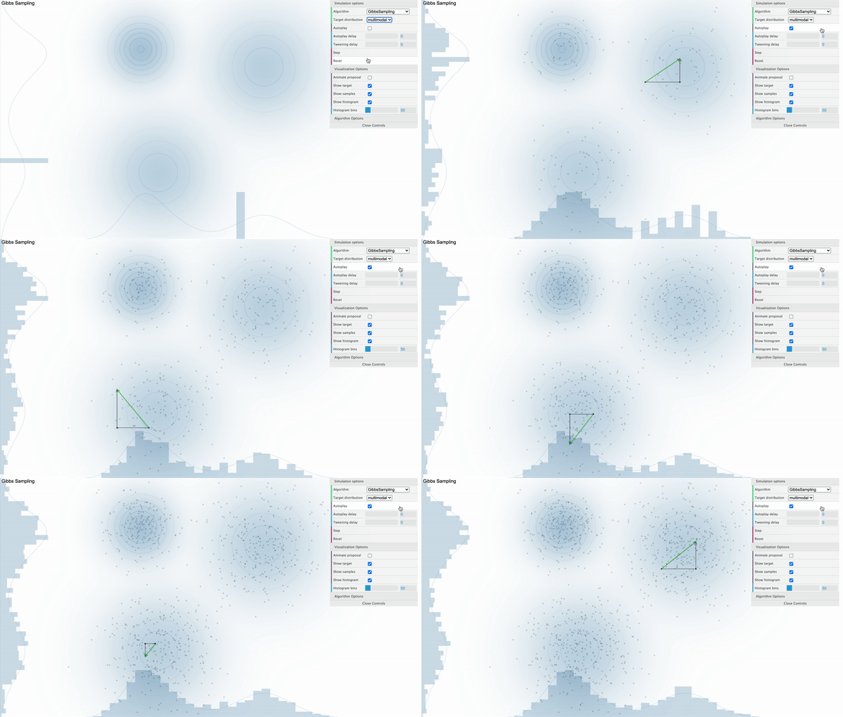
Gibbs Sampling
Unlike Metropolis-Hastings sampler where it got stuck on the local mode, It is clear that the Gibbs Sampler works well as samples are withdrawn randomly from various modes when we use Gibbs Sampler. Let’s talk about how this magic is done.
Steps of Gibbs Sampling
Let’s say that we are interested in evaluating the following posterior distribution.
Here, we have two parameters to be inferred and we will be using our samples to apply Monte-Carlo method. We will use Gibbs Sampler because applying Metropolis-Hastings for joint distribution of $\theta$ and $\phi$ is costly.
Here’s a simplification of the systematic-scan Gibbs Sampler algorithm, which is the basic Gibbs Sampler in practice.

Illustration of Gibbs Sampling Method
The above steps are nothing but simply evaluating one parameter at a time in a d-dimensional posterior distribution. Let’s take a close look at how it’s done.
<Step 1>
In the t-th state (iteration) of our Markov Chain, we have d number of parameters to be evaluated.
Firstly, we are going to sample $x_1^{t+1}$. To do this, we marginalize $x_1$ by every other parameters and define a conditional distribution as the following.
Then we sample $x_1^{t+1}$ from this conditional distribution. We have completed the sampling of a next state for a single parameter $x_1$.
- Next state samples: $x_1^{t+1}$
<Step 2>
As a next step we will sample $x_2^{t+1}$.
Likewise, we are going to marginalize every other parameters except for $x_2$ and get a conditional distribution. Note that we are using previously sampled $x_1^{t+1}$ instead of $x_1^t$.
Then we sample $x_2^{t+1}$ from this conditional distribution. So far, we have completed the sampling of two next state samples.
- Next state samples: $x_1^{t+1}, x_2^{t+1}$
Repeat the above procedure for each of the next $d-3$ parameters ${ x_3, x_4, … , x_{d-1} }$.
…
<Step d>
Lastly, we sample $x_d^{t+1}$ from the following conditional distribution.
Now we have the complete $d$ samples to be used for the $(t+1)th$ state!
- Final samples: $x_1^{t+1}, x_2^{t+1}, …, x_d^{t+1}$
Principles of Gibbs Sampling
In a nutshell, Gibbs Sampler works by repeating above steps. Then you might wonder how is decomposing the joint posterior into several pieces of conditional distributions possible. Here’s the reason why.
Above equation is from the <Step 1> of Gibbs Sampling process we previously looked at. Recall that our aim at this step is to sample $x_1^{t+1}$.
Here, it is evident that the joint posterior distribution (target distribution) on the left side can be decomposed into two parts by marginalizing $x_1$ out. However, since we are only interested in sampling $x_1$, and $x_2, x_3 , … , x_d$ are withdrawn samples from the last state, we can treat \(p(x_2,x_3,...x_d|y)\) as a deterministic variable that has nothing to do with our parameter of interest $x_1$.
Therefore, while sampling $x_1^{t+1}$, our target distribution is only proportional to the conditional distribution \(p(x_1|x_2,...,x_d,y)\) , which is formally called as the full conditional distribution for $x_1$.
An interesting point to note here is that all of the full conditional distributions for $x_1, x_2, … , x_d$ are defined from a single full poterior distribution. What this implies is that the full amount of information contained in the full posterior can be accounted by combining all of the individual pieces of information of the full conditional distributions together, which is again, the key idea of Gibbs Sampling algorithm.
For Gibbs Sampler to be used in practice, we just need one more condition. By now we know that Gibbs Sampling is a method that collects samples from the full conditional distributions. Regarding this, our full conditional distributions have to be defined as one of the standard probability distributions (ex. Gaussian, Gamma, Beta et cetera) in which we can generate random samples from. Otherwise, we cannot use Gibbs Sampler.
Example of Gibbs Sampling
Recall from the previous post that we wanted to find out the average height of male students in Yonsei university where the Bayesian setting was like the following. Note that prior of $\mu$ depends on $\sigma^2$, allowing information to flow between parameters in the hierarchical model.
Since our interest was on the average height of students, we wanted to get the posterior distribution of $\mu$ as the result of our Bayesian Inference. However, there was no way we could accomplish our goal because the posterior was not in a closed-form. Here’s as far as we went by analytical derivation.
Let’s see if we can solve this problem using Gibbs Sampling. Note that we are evaluating 2 parameters $\mu, \sigma^2$ at once. The key is to define the full conditional distributions.
Full Conditional Distribution of $\mu$
Let’s rewrite the joint posterior with respect to the parameter $\mu$.
- (A): removed all the terms that are independent of $\mu$
- (B): Rearranged the terms in quadratic order with respect to $\mu$
- (C): Added constant needed for square equation
As a result, we have the following full conditional distribution for parameter $\mu$ in the form of a normal distribution, which we can easily generate random samples from.
Full Conditional Distribution of $\sigma^2$
Likewise, we can derive the full conditional distribution for $\sigma^2$.
The final line of the equation holds by adding constant $\nu_o$ and $\beta_0$ to match the parameterization of inverse gamma distribution.
Since either of full conditional distributions for each parameters are defined as a standard probability distribution, we can use Gibbs Sampler to get posterior samples! It’s time to implement Gibbs Sampler using python.
Code implementation
Using our results, let’s define functions for each full conditional distributions.
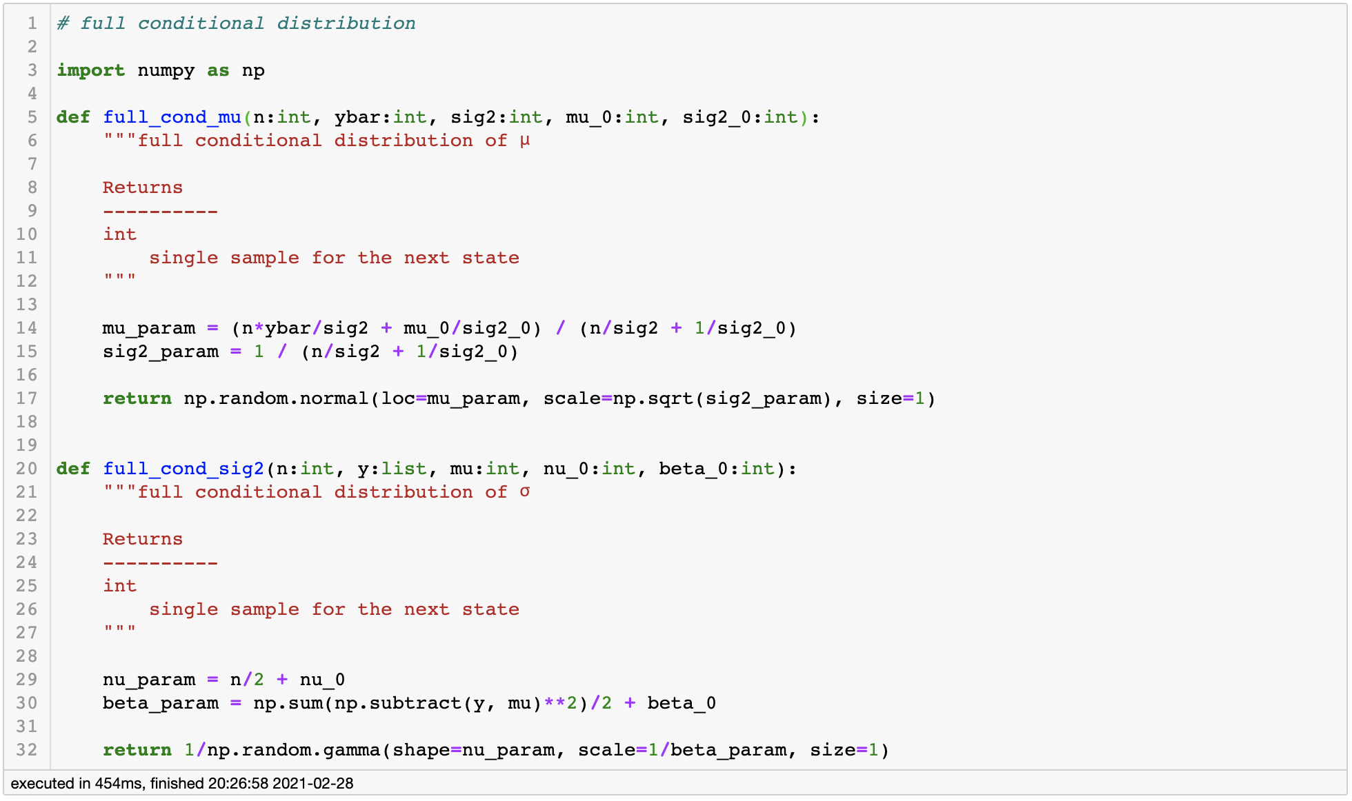
full conditional distribution
Then we will define the Gibbs sampler using above functions.
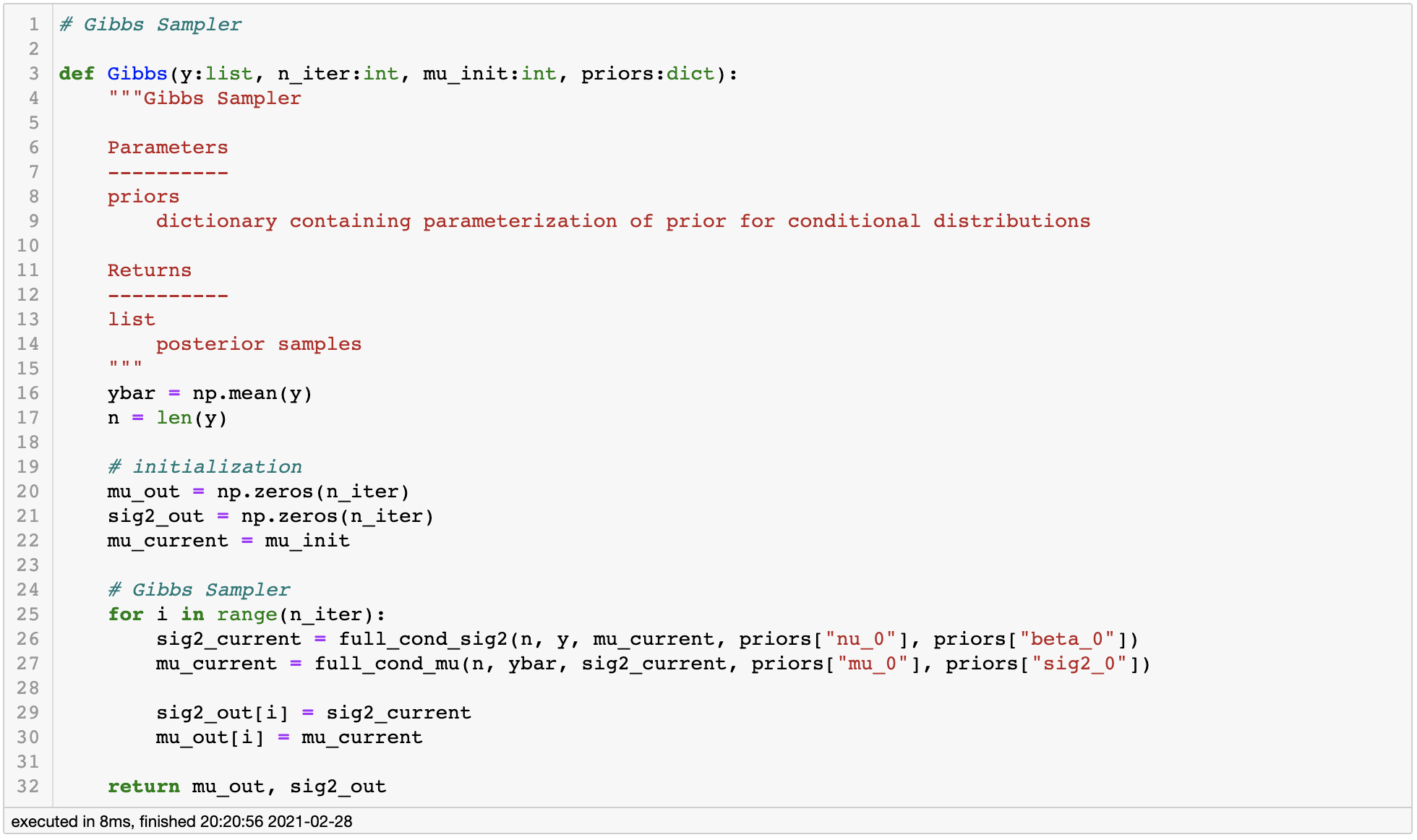
Gibbs sampler
Application
Now let’s check if our code works properly by plugging in some actual values to our example.
Suppose we have assumed that the average height of male students would roughly be around 175cm, with some amount of uncertainty enough to cover all the way from 160cm to 190cm. Note that we are using relatively informative prior because we have common sense on the height of male students - we know it can’t be something like 250cm. In situations where we don’t have any prior knowledge on the subject, we can use non-informative prior (or flat prior). The choice of the prior can be very sensitive especially when we have small observations so we always have to be ready for justification.
Here’s the visualization of our prior belief.
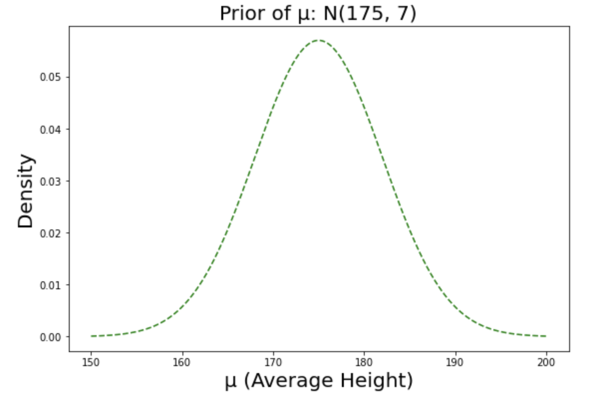
Prior distribution of $\mu$
In this setting, let’s suppose we interviewed 10 random male students and their height was [182.4, 188.1, 188.3, 185.2, 183.7, 192.5, 189.5, 188.7, 187.9, 186.3, 195.3, 189.4], which is generally larger than our prior belief of 175cm. If this was the case, we can intuitively guess that our posterior would have to move from 175cm to the observation mean 188.1cm. Let’s see if this actually happens.

Setting prior and likelihood
Just to make sure our Markov Chain converges to a proper stationary distribution, let’s initialize our Gibbs Sampler from 4 different starting points. If all of the chains converge to a similar point, we can say that we have correctly found the stationary distribution.
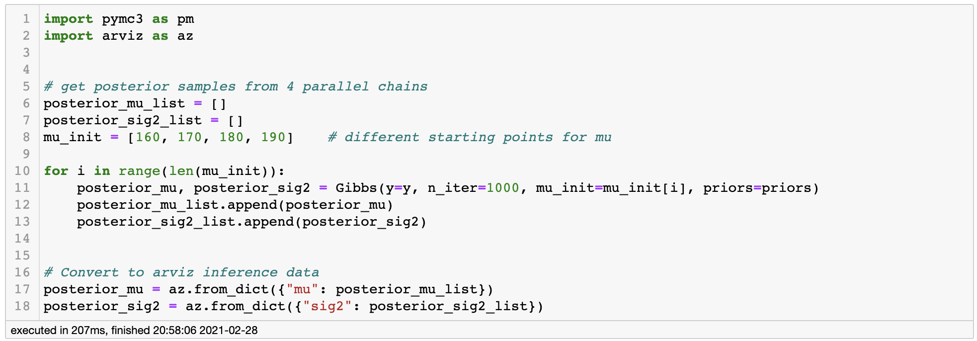
Running Gibbs Sampler
We can assess the convergence by plotting trace plot.

Trace Plot
It appears that all of the chains have converged to the same stationary distribution and the trace plot looks just fine. We can also use az.summary() function to get some numerical information of our posterior samples.

In the very right column we see rhat, which is a numerical measure of convergence. The closer it is to 1, the better the convergence. So by various evidence we can conclude that our samples have converged to the posterior distribution.
Posterior Analysis
As a last part, let’s diagnose the quality of our posterior samples.
For posterior inference, we normally have to discard some amount of the earlier samples as they can be inaccurate samples withdrawn from the Markov Chain that are yet to have converged. This is called as the burn-in period and in general we decide how many samples to be discarded by looking at the trace plot. For our example it would be unnecessary, but keep in mind that using earlier samples can possibly distort our inference.
For assessing the quality of our posterior samples, we will consider autocorrelation among the samples. Note that we have used Markov Chain so that our samples are inherently dependent on each other to some extent. Autocorrelation is a metric that measures the dependency among samples. If autocorrelation is close to zero, it means that the samples are independent, which is good thing.

Autocorrelation Plot
By autocorrelation plot, we can see that we have some amount of dependency among samples within 5~6 states. This is equivalent to saying that information is redundant among samples, hence it will reduce the amount of total information in our posterior samples. This is related to the concept effective sample size (ESS).

For our posterior samples, we have ESS of around 1490. What this means is that our withdrawn 4,000 MCMC samples contain information equivalent to that of 1490 i.i.d. samples from the true posterior distribution. I believe results inferred from Monte-Carlo estimation using 1490 samples is sufficient to be validified, so we can finally answer our original question.
Conclusion: Concerning 10 observed samples, average height of male students in Yonsei university is roughly around 185.7 cm.
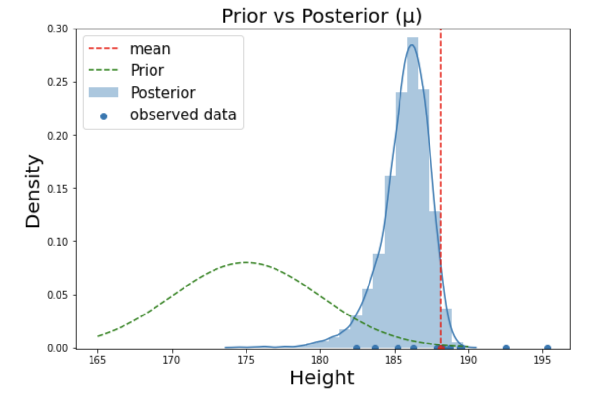
Result of Bayesian inference
It is interesting to see from the above figure that posterior is somewhere in the middle of prior and the observations. In fact, posterior is a compromise between prior and the likelihood. The amount being compromised depends on the amount of observations and information in the prior. That is, if we use highly informative prior with small amount of observation, our posterior will be formed closer to the prior distribution. On the other hand, if we have lots of samples say 100,000, our posterior will be pulled strongly closer to the observations with very high kurtosis (distribution is highly centered around the mean).
Remarks on Gibbs Sampling
Great. So we made it to the end of a full Bayesian inference using Gibbs Sampling. However, there is no free lunch as there are some obvious downsides of using the Gibbs Sampler.
Although it is really easy to implement and universally applicable, the most prevalent problem of Gibbs Sampler is that it produces highly correlated samples. Recall from our example that the effective sample size was less than half the size of our posterior samples. This can be troublesome as we are dealing with more complicated posteriors. In the worst scenario, the total information of our samples can be less than like 10% or even around 1~2%. If this is the case, we might have to withdraw millions of samples.
Moreover, as Gibbs sampling marginalizes the posterior by sequence of full conditional distributions, it consumes enormous amount of computer memory so inherently it is not suitable for large datasets. In general, batch training on Gibbs Sampler is inefficient, although there are some variations of Gibbs Sampling which makes it possible (for more information, check this article).
In the next post, we will take a look at the cutting edge MCMC algorithm HMC (Hamiltonian Monte Carlo) which can arguably overcome the limitations of Gibbs Sampling.
References
- https://chi-feng.github.io/mcmc-demo/
- Wikipedia: Gibbs Sampling
- Gelman et. al. 2013. Bayesian Data Analysis. 3rd ed. CRC Press.