[Bayesian Statistics] Hamiltonian Monte Carlo
This post is a gentle introduction to the Hamiltonian Monte Carlo, an highly efficient MCMC algorithm designed to overcome the weaknesses of Gibbs Sampling and Metropolis Hastings algorithm.
Previous Posts
1. Bayesian Statistics - Basics
2. Bayesian Statistics - Conjugacy
3. Bayesian Statistics - Hierarchical Models and Monte Carlo Simulation
4. Bayesian Statistics - Metropolis-Hastings
5. Bayesian Statistics - Gibbs Sampling
Overcoming MH & Gibbs
So far, we talked about Metropolis-Hastings algorithm and Gibbs Sampler as a roundabout solution for unsolvable posterior distributions. Although they worked well with our simple examples, problems exist when we want to deal with more complicated posteriors that are often high dimensional and correlated. Thus, we are going to take a look at a more advanced MCMC algorithm Hamiltonian Monte Carlo (HMC) , which extends to the state of the art MCMC sampling method No U-Turn Sampler (NUTS).
Before we talk about the details of HMC, let’s first justify the necessity of HMC in place of MH and Gibbs. By now we know how the latter two algorithms work to get samples from our target distribution - Metropolis Hastings uses random walk property of a Markov Chain and Gibbs Sampler uses conditional probabilities. However, this is where we might have to endure some possible inefficiency in the sampling process. For example when using a Metropolis Hastings algorithm, because the way how the samples are proposed is completely random, our sampler might re-explore the same points of target distribution over and over, making redundant and highly correlated samples. In general, this behaviour strongly reduces the acceptance rate of the MH algorithm for trickier target distributions, hence wasting lot time doing nothing at all.
The weakness of MH algorithm especially stands out for highly correlated target distribution. Let’s say that our target distribution is a donut-shaped and see how MH sampler performs.

[Fig. 1] Metropolis-Hastings
We can visually examine that most of the proposed samples are getting rejected and even for the accepted samples, they seem to be getting stucked locally. We can use reparameterization technic or effective jumping rules as a remedy but they do not fundamentally solve the problem of local random walk behaviour that is prevalent in high dimensional target distributions like the one above. This clearly urges the need for a more efficient sampling algorithm that produces more reliable samples.
Hamiltonian Monte Carlo
To reduce this local random walk behaviour of previous MCMC algorithms, Hamiltonian Monte Carlo (HMC) burrows a concept of “momentum” from physics. By including momentum variable $\phi$, the samples are withdrawn towards the direction of higher likelihood in the target distribution, rather than moving at random. This is made possible by using the concept of gradient. Recall that the gradient is a vector pointing towards the direction of the steepest (highest likelihood) slope at the current point.
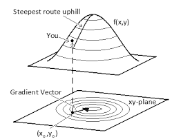
[Fig. 2] Geometric illustration of gradient vector
So in a nutshell, the direction of the HMC sampler is effected by the gradient of the log likelihood, allowing us to get reliable samples that realistically represents the target distribution. This might sound gibberish at the moment, so let’s take a look at the step by step details of HMC algorithm.
Leapfrog steps and momentum
In HMC, there are two key components to be kept in mind.
First, the leapfrog step ($L$) is the number of step that our sampler is allowed to explore the parameter space at a single iteration. Recall that in the MH and GIbbs sampler, the next state sample was a single move from the current state. In contrast, the next state of HMC sampler is the point moved $L$ times from the previous state. What this implies is that it allows the sampler to move farther in the parameter space where the path is governed by the likelihood of the target density. Thus during the $L$ steps in a single iteration, the movement of our sampler will be fully encouraged if it is going in the right direction, whereas the movement will be suppressed vice versa. Let’s visually examine this process.
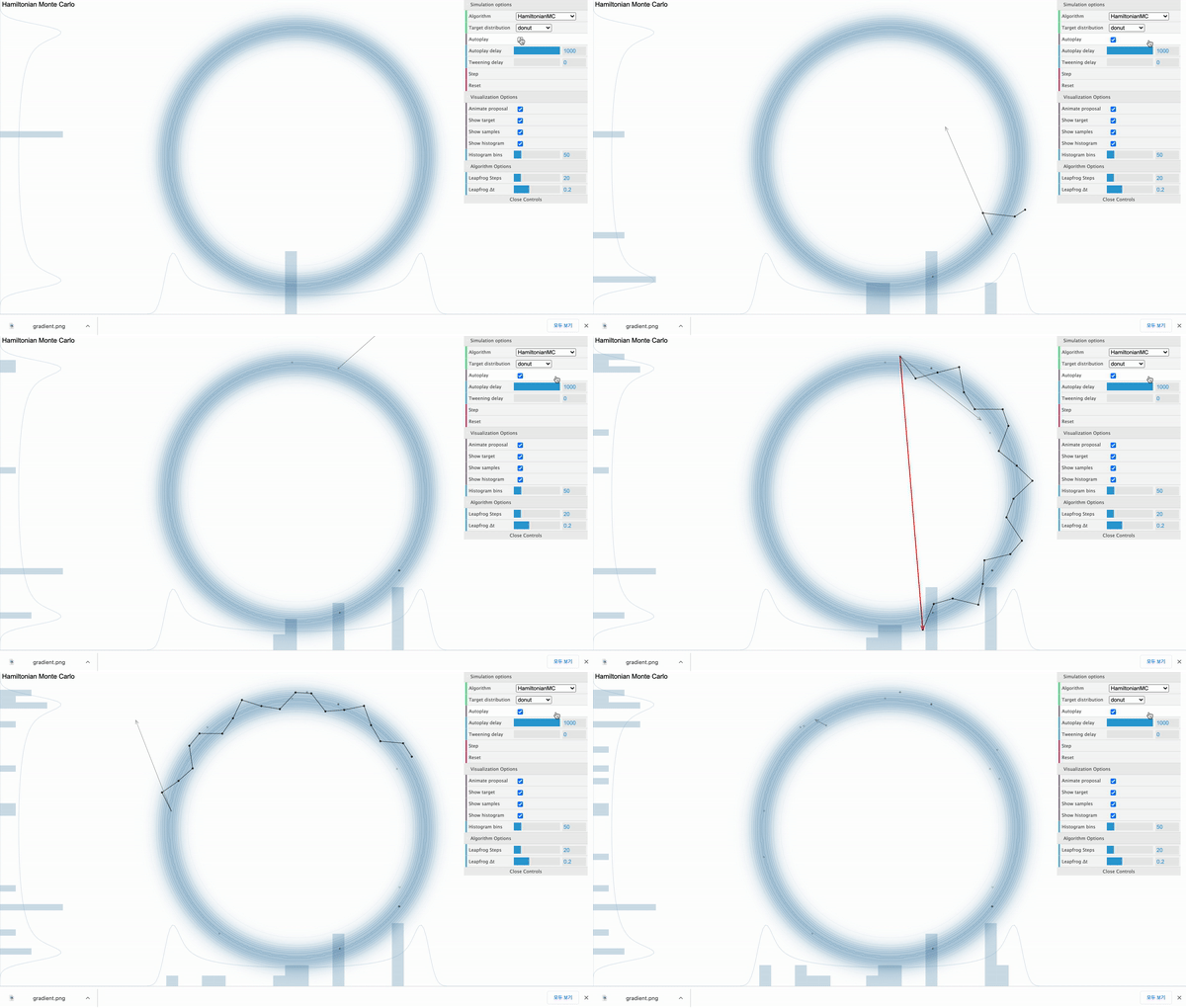
Hamiltonian Monte Carlo ( $L$ = 20 )
Above is the HMC sampler applied in the donut-shaped target distribution with leapfrog step size set to 20. For each iteration, the sampler can move 20 steps from the current position and its path is effected by the donut-shaped likelihood.
From above illustration, we can also see that the total distance moved differs from time to time. Regarding this, the momentum variable $\phi$ controls this distance. To be more specific, it controls the speed of movement in each steps. It is an auxiliary variable (hyperparameter) introduced to enhance the speed and efficiency of the sampling process, so $\phi$ is not a direct concern of our observation. In general, we assign multivariate normal distribution with diagonal covariance matrix as a prior distribution for $\phi$. It’s dimension ($d$) is the same as the number of parameters.
For implementation, the covariance matrix $M$ is set during the burn-in period and held fixed afterwards. Also, the posterior of $\phi$ is set to be the same as the prior for calculation simplicity.
Steps of Hamiltonian Monte Carlo
Now we are ready to talk about the nitty-gritty details of how sampling is done in HMC algorithm. Suppose we are at the i-th state of the sampling process with the parameter vector $\theta_i$ and momentum vector $\phi_i$.
<Step 1>
Randomly sample $\phi_i$ from its posterior distribution $N(0,M)$. This determines the initial direction of the sampler.
<Step 2>
With the predefined leapfrog step size $L$, sImultaneously update $\theta_i$ and $\phi_i$ for $L$ times.
(a) Update $\phi_i$
$\epsilon$ is an another hyperparameter that controls the amount of update. If you are familiar with Machine Learning models, it is similar to the learning rate.
(b) Update $\theta_i$
(c) Repeat (a) & (b) for remaining L-1 times.
By the end of this iteration, we will have next state candidate sample $\theta_i^*$ for our parameter.
Before we move on, let’s try to understand the intuition behind this updating procedure. Like I mentioned, $\phi$ is a variable indicating speed (momentum). Hence there are 3 possibilities of how the variables get updated with respect to $\phi$.
-
$\theta_i$ (position vector) is moving in relatively flat area of target density.
- If this is the case, \(\frac{d\;log\;p(\theta_i|y)}{d\theta_i} \approx 0\) and in (a), $\phi_i$ will not be updated at all. This is equivalent to saying that our sampler is moving at a constant speed.
-
$\theta_i$ is moving towards the sparser area of the target density.
- In this case, \(\frac{d\;log\;p(\theta_i|y)}{d\theta_i} < 0\) and $\phi_i$ will be decreased in (a). The decrease in the momentum will suppress our sampler’s movement to the current direction.
-
$\theta_i$ is moving towards the denser area of the target density.
- In this case, \(\frac{d\;log\;p(\theta_i|y)}{d\theta_i} > 0\) and $\phi_i$ will be increased, further speeding up the movement of our sampler to the current direction. The momentum will start to slow down after it passes the local mode.
<Step 3>
Using the candidate samples $\theta_i^{*}$ and $\phi_i^{*}$, calculate the acceptance ratio $r$.
- Before leapfrog step: $\;\theta_{i-1}, \; \phi_{i-1}$
- After leapfrog step: $\;\theta_i^{*}, \; \phi_i^{*}$
<Step 4>
Decide whether to accept/reject the candidate based on the acceptance ratio $r$.
Note that we do not record the update for the auxiliary variable $\phi$ since it is out of our interest.
Remarks on HMC
Hamiltonian Monte Carlo is designed to work with all positive, continuous target distributions. If at any point during an iteration the algorithm reaches a point of zero posterior density, the current step is discarded and the iteration restarts from the previous position, forcing the sampler to stay in the positive parameter space. Also it is proved that HMC preserves the detailed balance condition, thus our sampler is guarenteed to converge to the target distribution.
In case we are dealing with a constrained parameter, we can use transformation on the parameter such as the logit transformation for parameter space in [0, 1] and log transformation for parameter constrained to be positive. Moreover for the discrete parameter space, we can think of using poisson regression.
For the last part, emphirical results tell us that the optimal acceptance ratio should be somewhere close to 65% (Note that this specific value is just a rough guideline!). Thus when implementing HMC in practice, it’s typical to set the hyperparameter $\epsilon$ and $L$ with the condition $\epsilon L = 1$. Based on this condition, for too small acceptance ratio we should increase $\epsilon$ as it controls the amount of update. Intuitively, small $\epsilon$ indicates that our sampler will take small steps for its movement in the parameter space meaning that it is moving cautiously. On the other hand, if the acceptance ratio is too big, then we should consider decreasing $\epsilon$, allowing our sampler to take relatively ambitious steps in the parameter space.
No U-Turn Sampler (NUTS)
As the last part of this post I will briefly mention about the NUTS, which is the mostly widely used MCMC algorithm in practice. As a matter of fact, it is a default MCMC sampler for continuous posterior densities in pymc3.
So it is easy to think of the NUTS as an improved version of HMC, with the biggest improvement being that the leapfrog step size $L$ is determined automatically. Because we had to manually define the number of leapfrog steps (iterations), in case if it is set too large then our sampler might eventually return to the nearby area where it started (see below illustration taken from this blog).
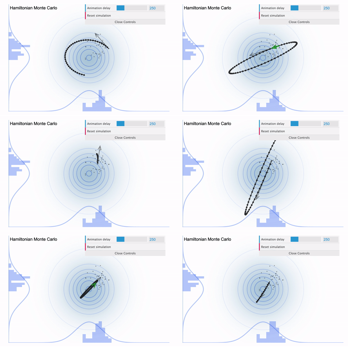
Hamiltonian Monte Carlo with large L
To address this issue, NUTS allows the sampler to travel as far as it can go and when the sampler trys to make U-turn it stops the iteration. In a mathematical sense, this U-turn is equvalent to when the inner product of the momentum variable $\phi$ and the position vector $\theta$ becomes negative. As a matter of fact, NUTS is a lot more trickier and sophisticated algorithm. So in addition to the U-turn property, NUTS has some additional settings to make it satisfy the detailed balance condition and the hyperparameters are defined during the burn-in period and fixed afterwards. Below is an illustration of the NUTS sampler in practice.
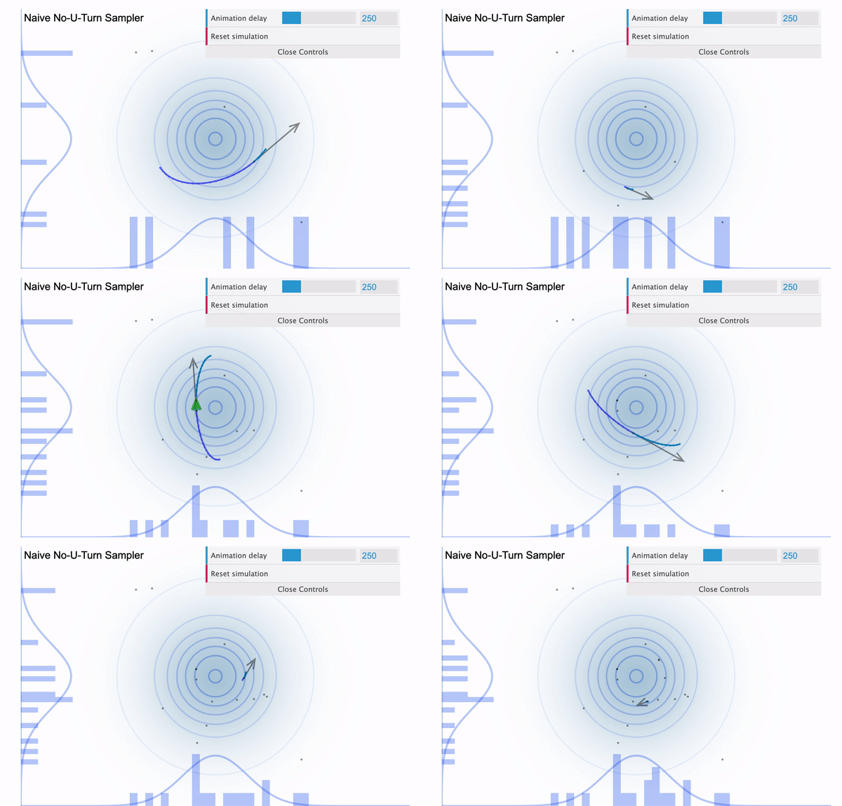
No U-Turn Sampler
Hence as long as we don’t have any clear reason to use other MCMC samplers, it is always better and safe to use NUTS for withdrawing samples for our posteriors as pymc3 makes everything handy for us.
References
- https://chi-feng.github.io/mcmc-demo/
- Wikipedia: HMC
- http://elevanth.org/blog/2017/11/28/build-a-better-markov-chain/
- Gelman et. al. 2013. Bayesian Data Analysis. 3rd ed. CRC Press.