Ch1. Introduction to Spatial Data
In this post, we will take a look at some of the basic concepts necessary for analyzing spatial data.
Contents
Challenges of Spatial Data
For traditional statistical inferences, data are assumed to follow i.i.d. condition (independent + identically distributed).
However in spatial data, data are very rarely i.i.d. because they are geographically referenced. That is, data are spatially dependent. Thus, we have to come up with more complex models that can account for this covariance structure.
Overlooking this dependency might lead to poor estimates and prediction because of the underestimated variance.
- Variance estimation with i.i.d assumption
-
Variance estimation with covariance structure $Cov(Z_i, Z_j) = \sigma^2 \rho^{\lvert i - j \rvert}$
We can see from the equation that for stronger covariance (large $\rho$), the estimated variance is larger than $\frac{\sigma^2}{n}$.
Here, $\; n^* = \Big( 1 + 2(\frac{\rho}{1-\rho})(1-\frac{1}{n}) - 2(\frac{\rho}{1-\rho})^2 (\frac{1-\rho^{n-1}}{n}) \Big)$ is called as effective sample size. Note that for sufficiently large $n$, $\; n^* \rightarrow n \Big( \frac{1-\rho}{1+\rho} \Big)$, which indicates that even in asymptotical sense the variance structure still exists.
One advantage of modeling spatial dependency structure is that sometimes overlooked covariates can be adjusted by spatially dependent error term $\epsilon$. But the problem is that modeling this spatial dependency structure is often burdensome.. For one reason, the dependency may be present in all directions. Thus to make long story short, a convenient solution is to decompose the model into two part - mean structure & covariance structure.
-
For the covariance structure, it seems natural to assume that the correlation between two points deminish along with the distances. In other words, data that are further apart are less dependent than the data located nearby. We can use various covariance functions for this purpose.
-
For modeling the mean structure, Gaussian Process is often utilized.
In this sense, spatial data analysis (modeling) is built on top of existing methodologies. For example, Bayesian Hierarchical Models and computation is used to define a spatial model, Gaussian Process is used to model the mean structure, Markov Random Field is used for modeling the correlation structure and the concept of distance is rendered for analyzing spatial data.
We will take a look at how these can be implemented in the subsequent posts.
Types of Spatial Data
Let’s denote spatial data in $d$ dimensions (usually $d=2$) by \(\{ Z(s) : s \in D \subset R^d \}\) , where $s$ is the geographical location where the process $Z(s)$ is observed.
In general, spatial data can be characterized into the following 3 categories:
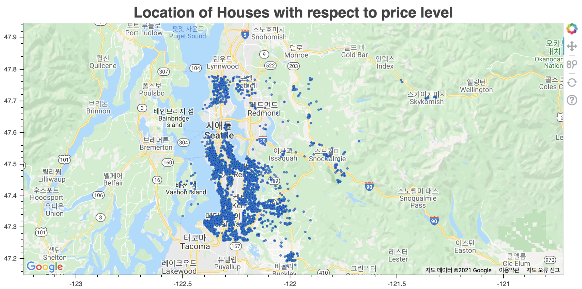
1. Geostatistical Data
- A spatial process which is observed only at points (usually coordinates).
- ex) PM 2.5 concentration in Seoul
- $D$ is a continuous fixed set.

Example of Geostatistical Data
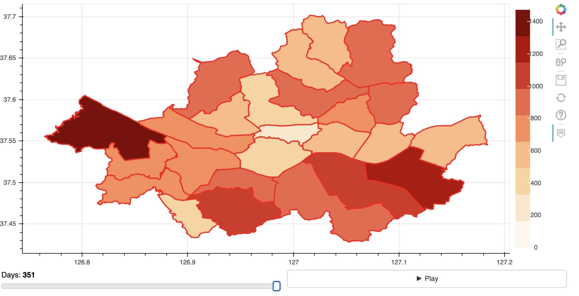
2. Lattice (Areal) Data
- A spatial process which is observed at a discrete level (countably many locations).
- This usually arises as a result of aggregation like daily COVID-19 infection counts for different countries.
- $D$ is a discrete fixed set.
- Because the data are aggregated by a unit location, the data may be more complete compared to geostatistical data.

Example of Lattice Data
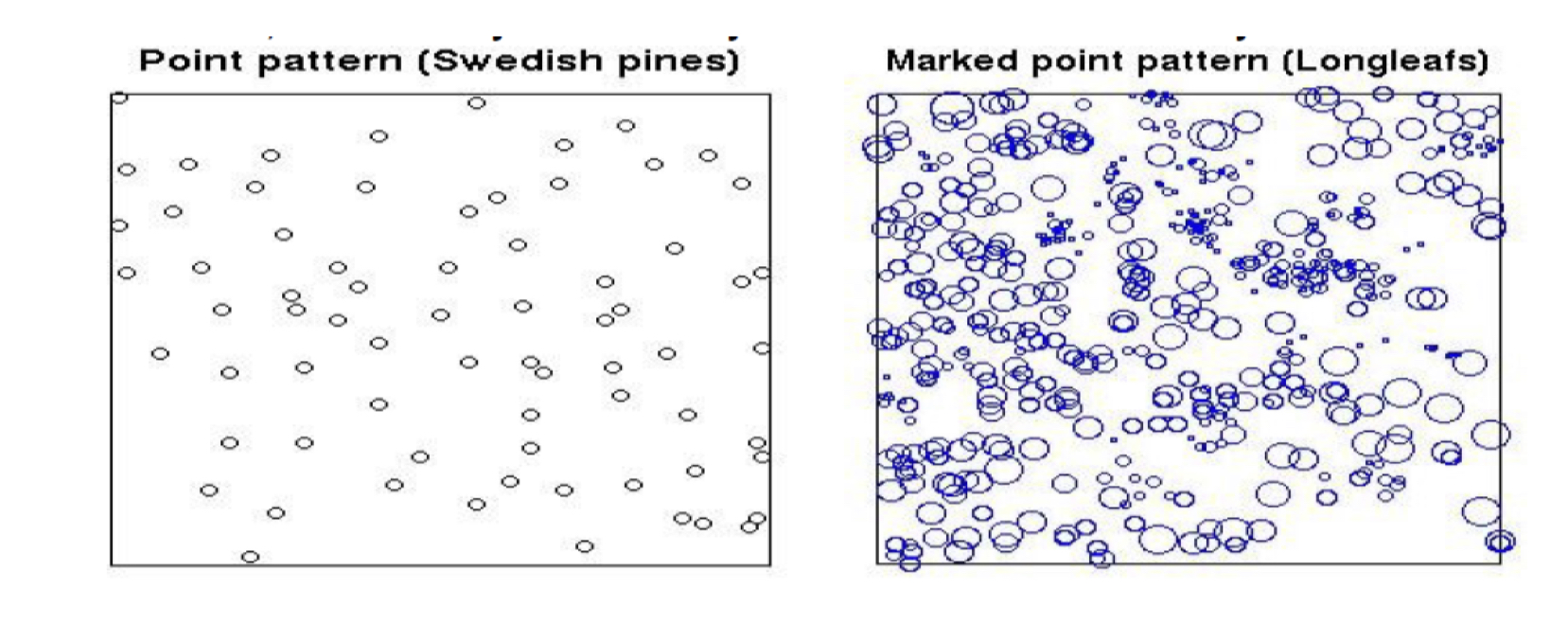
3. Spatial Point Process
- A spatial process is observed at points, but the locations are of interest on their own.
- A naive example is the case where we are interested in the clustering patterns among spatial data points.
- $D$ is stochastic, typically continuous.
- We are often interested in finding out the spatial clusters, where each unit location has its own mean and variance structure.

Example of Spatial Point Process (from Baddeley and Turner R package, 2006)
Characteristics of Spatial Data
Some of the distinctive characteristics of spatial data are as follows:
- We are mostly interested in interpolation (what happens at unobserved locations between geographical points). It’s easy to think of this as a prediction for spatial dataset. I think this term is due to the philosophical discipline of spatial data analysis field.
- In comparison to the asymptotic (large sample) theory in classical statistics, spatial data analysis assumes increasing domain asymptotics, where our focus is to find out what happens as the domain gets bigger (like the accuracy of interpolation).
- Spatial process often only have a single realized value of $n$ x $1$ vector. That is, we treat the $n$ data points at the same time. If the data is logitudinal over time, then we can have several replicates ($n$ x $p$).
- In addition to the spatially dependent structure, the predictor and response variables are often highly multivariate and correlated which necessitates hierarchical models.
- Some additional difficulties arise due to Non-Gaussian structure and Misalignment of data points. Misalignment refers to the problem when the domain of predictor doesn’t correspond to the response variable (e.g. predictor variables collected at a county level, but the response is at a country level).
Some Prerequisite Knowledges
We need some background knowledges in order to understand and implement spatial data analysis.
1. Notion of Distance
The most simplest metric of measuring the distance between two points is the Euclidean Distance.
In spatial dataset however, there is a problem of using Euclidean Distance because it ignores the curvature of Earth. In turn, the actual distance between two points on Earth’s surface will be distorted if we naively use the Euclidean Distance.
As a remedy, Geodesic Distance or Chordal Distance is often used as a more realistical measure of distance for spatial data.
<Geodesic Distance>
\(D_{Geo} = R \arccos{[\sin(lat1) \sin(lat2) + \cos(lat1)\cos(lat2)(lon1-lon2)]}\)
<Chordal Distance>
\(\begin{aligned} &x_i = R \cos(lat_i) \cos(lon_i) \\[10pt] &y_i = R \cos(lat_i)\sin(lon_i) \\[10pt] &z_i = R\sin(lat_i) \\[10pt] &u_1 = (x_1, y_1, z_2), \quad u_2 = (x_2, y_2, z_2) \\[10pt] &D_{Chor} = D_{Euc}(u_1, u_2) \end{aligned}\)
where $R = 6371$ is the mean radius of Earth in km. Note that the Chordal DIstance is a Euclidean Distance for $R^3$.
2. Gaussian Process
A Gaussian Process is a stochastic process whose finite-dimensional distributions of each states are all multivariate gaussians. Since we are dealing with spatial data, a spatial stochastic process can be represented by the collection of random variables such that
where $s$ indicates individual locations and $Y(s)$ is the corresponding observation (for a spatial process, we typically have a vector $Y = (Y(s_1), Y(s_2), … , Y(S_n))^\prime$ of $n$ observations).
Since Gaussian Process is a stochastic set of finite Gaussian variables, we only need to define the mean and covariance structure in order to fully define a Gaussian Process.
where $C(s_i, s_j)$ is often characterized by various covariance functions.
A famous covariance function for modeling the spatial dependency is the Matérn covariance function given by
where $\nu$ is the smoothness parameter that controls the differentiability of a Process with Matérn covariance and $K_\nu$ is a Bessel function of order $\nu$. For our purposes, I think it is sufficient to know that we can use this function for the covariance structure rather than the nitty-gritty details of its components.
3. Isotropy
For the covariance structure of a spatial process, it is often assumed to have isotrophic characteristics. This means that the covariance (or more generally any attributes) only depends on the distance of two points and invariant to the direction.
This concept is related to the property of stationarity in a (spatial) stochastic process such that for any set of observations $Y(s_1), \dots, Y(s_n)$ and any spatial lag $h$, we have
This is called as a strong stationarity. A slightly weakened variation of this condition is
which is called as a second-order(weak) stationarity defined by the moments of spatial random variable $Y$.
- Note that for a Gaussian Process, the strong stationarity and weak stationarity are equivalent because the two moments are sufficient to fully define a stochastic process.
By taking a step further, a second-order stationarity of a process implies a intrinsic stationarity, which is $Var[Y(s+h) - Y(s)]$ depending only on the lag $h$. When this condition is satisfied, we can define a function of lag $h$ such as
and we call this function as a variogram. This variogram is generally utilized for diagnosing the existence of spatial dependency among the points in the dataset.
- As a reminder, second-order stationarity implies intrinsic stationarity but not the other way around.
Therefore, regarding spatial data analysis and modeling, we can now answer the following questions:
- How can we define distance?
- How can we measure spatial dependency?
- How to perform EDA for a spatial data?
With this in mind, we will see how we can actually implement statistical inference for spatial data in the subsequent post.
Reference
This post is written based on the lecture note of Spatial Data Analysis (STA6241), held at the Department of Statistics & Data Science at Yonsei University 2021-2 autumn semester.