Ch2. Classic Geostatistical Inferences

2021, Oct 07

In this post, we will take a look at the details of classic statistical inference for geostatistical (point-referenced) dataset. Specifically, we will see the outlines of parameter estimation and prediction for spatial model with Gaussian Process, along with implementation on a real dataset using R.

 

Contents

1. Goals of Statistical Inference
2. Model Specification
3. Parameter Estimation
4. Krigging

 

---

Goals of Statistical Inference

 

Roughly speaking, there are two main goals we are concerned with when making inference about spatial data (or more broadly any kind of data domain).

• To make inference about data generating process
  • This is equivalent to specifying a model to be used, which is accomplished by estimating its parameters.
• To predict $Y(S_{new})$ for new data point $S_{new}$
  • For spatial domain, this is called as interpolation (or krigging)

 

Therefore, the very first step of data analysis is to define a (parametric) model.

 

---

Model Specification

 

With the assumptions of stationarity and isotropy, let’s define a spatial model such that:

 

$$ \begin{aligned} Y(s) &= \mu(s) + \eta(s) + \epsilon(s) \\ \; \\ \; \\ \mu(s) = E[Y(s)] = X^\prime\beta &: \quad \text{Deterministic Linear Mean Trend} \\[10pt] \eta(s) \sim GP\big(\textbf0, \sigma^2 \Gamma(\rho) \big) &: \quad \text{Spatially-correlated Gaussian Process} \\[10pt] \epsilon(s) \sim N\big(\textbf0, \tau^2I_p \big) &: \quad \text{White Noise Process of Measurement Error} \end{aligned} $$

 

where $\sigma^2$ is the overall variance of spatial points, $\rho$ is the dependency parameter and $\tau^2$ is the nugget (error).

• Note that there are four parameters to estimate in this model which are ${ \beta, \sigma^2, \rho, \tau^2 }$.

In this sense, the reason of modeling correlation structure by Gaussian Process is because it is easy to handle. Namely, we can use the desirable property of Gaussian distributions such that the marginal and conditional distributions of multivariate Gaussian random variables are also Gaussian, and since we only need two parameters (mean, covariance) for the Gaussian Process parameter estimation is greatly simplified.

However, there are some shortcomings as well especially in terms of computational costs as we have to derive the inverse matrix of the covariance function from the likelihood kernel \((\bf y- \bf \mu)^\prime\Sigma^{-1}(\bf y- \bf{\mu})\) . It is generally known that the complexity is of order $O(n^3)$.

Anyways, Gaussian Process usually provides reasonable fit for spatial dependencies, so unless we have any critical objections we will stick to it.

 

---

Parameter Estimation

 

In this part, we will first take a look the classical geostatistical approach of estimating model parameters.

In a nutshell, it can be abstracted as the following steps:

1. Get preliminary estimate of $\hat \beta_{OLS}$ using the least squares method.

2. Using the residuals from the preliminary estimate, estimate the variance components $\sigma^2, \rho, \tau^2$ with variogram and diagnose the dependency structure.

3. Re-estimate $\beta$ by generalized least squares method using the estimated variance components ($\hat \beta_{GLS}$)

 

As a result, we can fully define our model and in turn we can perform krigging (prediction) for unobserved points.

However, note that this estimation procedure doesn’t provide optimal estimate of the parameters because the parameter estimation is sequential and we cannot assess uncertainty of our estimators. Nevertheless, it can still be useful for the EDA steps such as finding out the clustering patterns among geological points. A more ideal alternative of parameter estimation is to use Bayesian methodologies, which will be introduced in subsequent lectures.

 

Anyways, let’s dig into the details of each steps. For a concrete illustration, we are going to actually implement these steps in R using the temperature data of California.

 

Dataset

The dataset CAtemps.RData contains two R objects of class SpatialPointsDataFrame, namely CAtemp and CAgrid where CAtemp contains information about average temperatures (in degrees Fahrenheit) of 200 locations in California from 1961-1990 along with their elevations in meters.

 

Overview of CAtemp Dataset

 

Using this dataset, our goal is to fit a spatial model for average temperatures where the model can be defined as the following:

 

$$ \begin{aligned} &Y_i = \mu(s_i;\beta) + e(s_i;\sigma^2, \rho) + \epsilon_i, \\[10pt] \; \\ \text{where }\;\; &\mu(s_i;\beta) = \beta_0 + \beta_1 Longitude(s_i) + \beta_2 Latitude(s_i) + \beta_3 Elevation(s_i) \\[10pt] &e(s_i;\sigma^2, \rho) : \text{mean zero Gaussian Process} \\[10pt] &e_i \sim N(0,\tau^2): \text{nugget (measurement error)} \end{aligned} $$

 

In this setting, we are going estimate the model parameters using CAtemp and perform krigging for unobserved locations in CAgrid by the fitted model.

 

Step 1. Preliminary Estimate of $\beta$

The ordinary least squares estimate of $\beta$ is by definition which minimizes

$$ \hat \beta_{OLS} = \underset{\beta}{argmin} (Y-X\beta)^\prime (Y-X\beta) $$

where $X$ is a $n$ x $p$ design matrix.

From this, we can derive the estimate of $\beta$ such that

$$ \hat \beta_{OLS} = (X^\prime X)^{-1}X^\prime Y $$

and the corresponding residual vector $\hat \epsilon$ is

$$ \hat \epsilon = Y - X\hat \beta_{OLS} $$

 

 

Let’s visualize the residual plot.

 

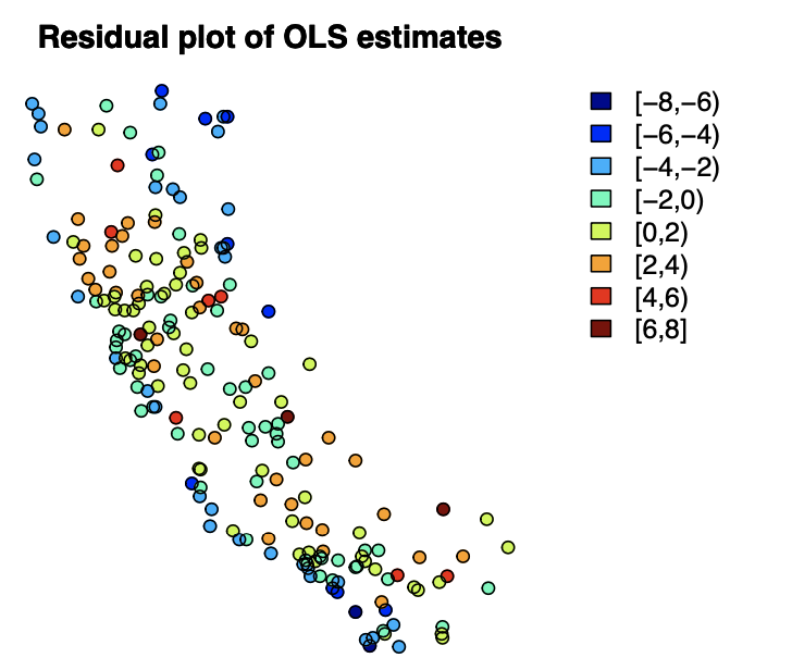
There seem to be some possible correlation structure among the residuals with respect to geological locations. This can more formally be determined by the variogram.

 

Step 2. Fit variogram and estimate the variance parameters $\sigma^2, \rho, \tau^2$

For two different spatial points $s_i$ and $s_j$ with a lag $h$, a variogram is defined as

 

$$ \begin{aligned} \gamma(h) &= \frac{1}{2} Var(e(s+h) - e(s)) \\[10pt] &=\frac{1}{2} E\big[ \big(e(s+h)-e(s)\big)^2 \big] \quad \because E\big[e(s+h) \big] = E\big[e(s) \big] = 0 \\[10pt] &\text{where } e(s) = \eta(s) + \epsilon(s) \end{aligned} $$

 

Since we only have a single realized value of temperatures, we don’t have replications of the lag $h$. Nevertheless, we can bin our dataset into several lags and get the estimated variogram by the method of moments such that

 

$$ \hat \gamma(h_u) = \frac{1}{2 \; \#\{s_i - s_j \in H_u\}} \sum_{s_i-s_j\in H_u} \big[ \hat e(s_i) - \hat e(s_j) \big]^2 $$

 

where the symbol # indicates number of elements in a specific set and $H_u$ is the partition of the space by lag $u$.

Let’s fit an exponential variogram using our dataset.

 

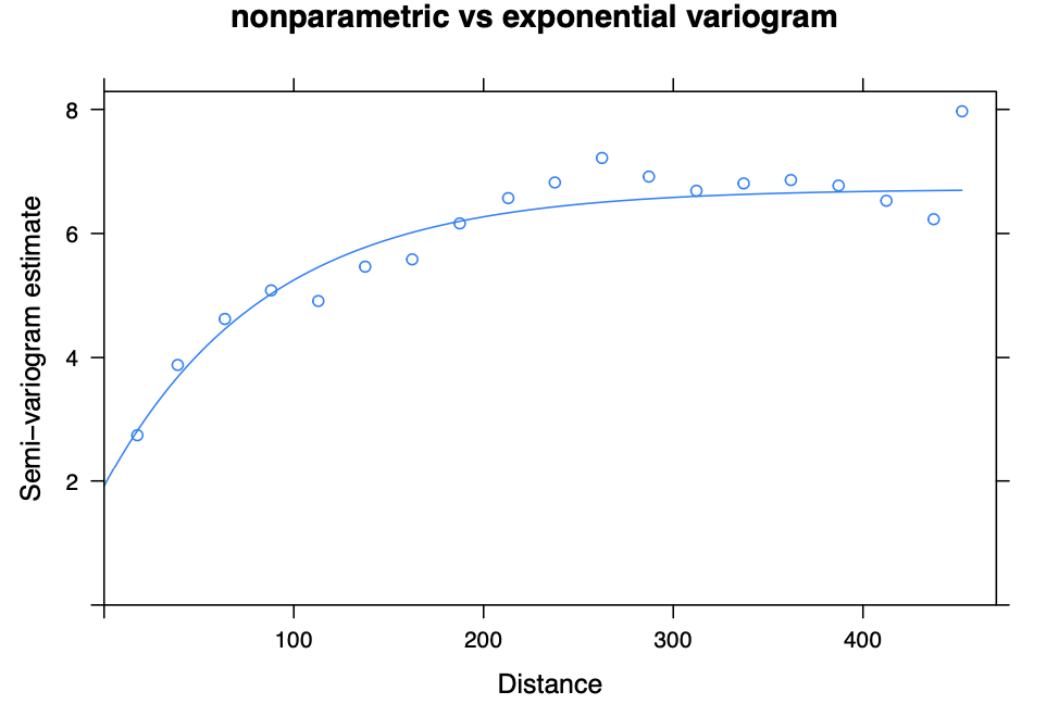
By the fitted variogram, we can see that there is some dependency structure with respect to the spatial lags.

The reason for using parametric variogram like the exponential is because we are going to estimate the variance parameters $\sigma^2, \rho, \tau^2$ using the fitted variogram. In this case, because the parameters are constrained to form a covariance matrix of the Gaussian Process which must be positive (semi) definite, we are using covariance functions that satisfies this condition.

Anyways, if we have successfully fitted a parametric variogram, then we can derive the weighted least squares estimate of the variance components \(\hat \theta_{WLS} = \{\hat \sigma^2, \hat \rho, \hat \tau^2\}\) such that

 

$$ \hat \theta_{WLS} = \underset{\theta = \{\sigma^2, \rho, \tau^2 \}}{argmin} \sum_{u} \frac{\#\{ s_i - s_j \in H_u \}}{\gamma(h_u;\theta)^2} \big[ \hat \gamma(h_u) - \gamma(h_i;\theta) \big]^2 $$

 

where for our example is calculated and stored in the variables sigma2_hat, rho_hat and tau2_hat.

 

Step 3. Re-estimate $\beta$

Finally, we can re-estimate the mean trend parameter $\beta$ by the generalized least squares method using the variance parameters we have estimated in step 2.

$$ \begin{aligned} \hat \beta_{GLS} = \big( X^\prime \hat \Sigma^{-1}X \big)^{-1} X^\prime \hat\Sigma^{-1}Y, \quad (\hat\Sigma^{-1} \text{ is the estimated covariance matrix}) \end{aligned} $$

 

To implement this in R, we have to first define a distance matrix among the locations in our dataset. Then, we will define the covariance structure by using the exponential covariance function and get the estimated covariance matrix $\hat \Sigma^{-1}$

Note that the exponential covariance function is defined as the following formula:

$$ \gamma(h) = \sigma^2exp\big(\frac{-\left\| h \right\|}{\rho} \big) $$

where $\lvert\lvert h \rvert\rvert$ is the distance matrix.

 

Now we are ready to derive $\hat \beta_{GLS}$.

 

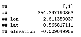
Finally, we have completely defined our model!

 

---

Krigging

As a next step, it’s time to get predictions for unobserved locations. In a spatial analysis domain, the prediction for unobserved location is called as krigging (or interpolation) so I will stick to the term krigging.

Since we have defined our covariance structure by the Gaussian Process, we can use the decent property of multivariate normal distribution that the conditional and marginal distribution can be factorized as

 

$$ \begin{aligned} {Y_1 \choose Y_2} \sim N\Big( {\mu_1 \choose \mu_2}, &\begin{pmatrix} \Sigma_{11} & \Sigma_{12} \\ \Sigma_{21} & \Sigma_{22} \\ \end{pmatrix} \Big) \\[20pt] \text{where }&Y_1 \sim N \big(\mu_1, \Sigma_{11} \big) \\[10pt] &Y_2 |Y_1 \sim N \big(\mu_2 + \Sigma_{21} \Sigma_{11}^{-1}(Y_1 - \mu_1),\; \Sigma_{22} - \Sigma_{21}\Sigma_{11}^{-1} \Sigma_{12} \big) \end{aligned} $$

 

Using this property, we can define the joint distribution of $Y$ and $Y(s_0)$ as

 

$$ \begin{aligned} {Y \choose Y(s_0)} \sim N\Big( {m \choose m_0}, &\begin{pmatrix} \Sigma & \gamma \\ \gamma^\prime & \sigma^2 \\ \end{pmatrix} \Big) \\[20pt] \end{aligned} $$

 

In this setting, let \(\hat Y(s_0) = \lambda_0 + \lambda^\prime Y\) indicate the krigging vector.

if we assume $\lambda_0 = m_0 - \lambda^\prime m$, then we have

$$ \begin{aligned} E[\hat Y(s_0) - Y(s_0)] &= E[\lambda_0 + \lambda^\prime Y - Y(s_0)]\\[10pt] &= 0 \end{aligned} $$

which implies the unbiasedness of the krigging estimator.

Therefore, to get the BLUP (Best Linear Unbiased Predictor) of $Y(s_0)$, it is natural to search for an estimator that minimizes the variance such that

$$ \begin{aligned} \hat \lambda_{opt} &= \underset{\lambda}{argmin} \; Var\big( \hat Y(s_0) - Y(s_0) \big)\\ &= \underset{\lambda}{argmin} \; Var\big( \hat Y(s_0)\big) + Var\big(Y(s_0) \big) -2Cov(\hat Y(s_0), Y(s_0)) \\[10pt] &= \underset{\lambda}{argmin} \; \{ \lambda^\prime \Sigma\lambda + \sigma^2-2\lambda^\prime\gamma \} \\[10pt] &\Leftrightarrow \frac{\partial}{\partial \lambda} \{ \lambda^\prime \Sigma\lambda + \sigma^2-2\lambda^\prime\gamma \} \overset{set}{\equiv} 0 \\[10pt] &\therefore \hat \lambda_{opt} =\Sigma^{-1}\gamma \\[10pt] &\Rightarrow\hat Y(s_0) = m_0 + \gamma^\prime \Sigma^{-1}(Y-m) \end{aligned} $$

 

The derivation of the krigging estimator from the above equation assumes that we know the values of the parameters of the joint normal distribution. However, in realistic situations, we often don’t know the mean parameters $m$ and $m_0$ as well as the covariance parameters $\theta = (\gamma, \sigma^2)$.

Therefore, we have to somehow estimate these parameters by our dataset and plug in the estimated parameters to get the krigging values. The krigging estimator defined by this is called as the EBLUP (empirical BLUP). The EBLUP tends to underestimate the true error because it ignores the variability coming from estimating $\theta$ in the first place, which leads to lower performance. In subsequent posts, we will see how Bayesian methods can solve all of these problems completely.

 

Krigging Example

Now let’s implement the above illustration of krigging for our CAgrid dataset.

First, we have to define distance matrix and derive the covariance matrix. Note that we are trying to derive the “EBLUP” by reusing the estimates from previous questions since we have no idea about the parameters.

 

And we are ready to get the predictions.

$$ \hat Y(s_0) = X(s_0)^{\prime} \hat\beta_{GLS} + \gamma^{\prime}\Sigma^{-1}(Y-X^\prime\hat\beta_{GLS}) $$

 

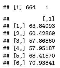
Furthermore, we can calculate the mean squared error for our predictions by the following formula:

$$ MSE(s_0) = \sigma^2 - \gamma^{\prime} \Sigma^{-1}\gamma + b^{\prime}(X^{\prime}\Sigma^{-1}X)^{-1}b,\\ where\;\;\;\;b = X(s_0)^{\prime} - X^{\prime}\Sigma^{-1}\gamma $$

 

Let’s visualize the predictions and standard errors.

 

 

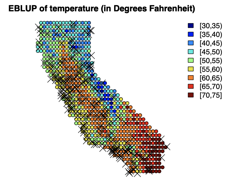
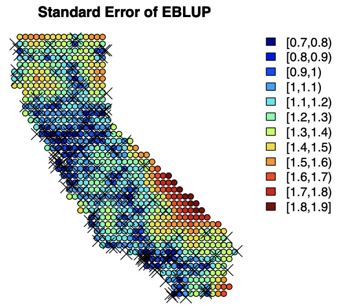
From the plot of standard errors, we can see that the error is relatively small for locations with lots of nearby data points which seems reasonable.

---

Reference

This post is written based on the lecture note of Spatial Data Analysis (STA6241), held at the Department of Statistics & Data Science at Yonsei University 2021-2 autumn semester.