[Bayesian Statistics] Basis Function Models

2021, Oct 26

 

Ch 20. Basis Function Models

This post is a summary of Chapter 20 of the textbook Bayesian Data Analysis.

---

Table of Contents

20.0 Nonparametric Models

20.1 Splines and weighted sums of basis functions

20.2 Basis selection and shrinkage of coefficients

20.3 Non-normal models and multivariate regression surfaces

 

20.0 Nonparametric Models

• Chapter 19 dealt with “parametric” nonlinear models where the function of predictors and parameters were prespecified.

$$ \begin{aligned} E[y|X, \beta] = \mu(X_i, \phi) \end{aligned} $$

• In the following chapters, we consider models where the function $\mu$ is also a priori unknown.

• Since we don’t know $\mu$, we have to estimate it somehow.
• There are various ways to model $\mu$ and in this chapter, we consider using basis function expansions.
• The key idea of basis function models is to linearly combine set of simple functions of the predictor variables to approximate arbitrary nonlinear functions.

$$ \begin{aligned} y_i = w_0\phi_0(1) +w_1\phi_1(x_{i1}) + \dots + w_n\phi_n(x_{in}) \end{aligned} $$

• Note that above equation reduces to standard linear regression model when $\phi$ is an identity function.

 

---

20.1 Splines and weighted sums of basis functions

 

Basis Function Expansion

Let’s consider a set of nonlinear functions $\mu(\dot)$. We can model this $\mu$ by the basis function expansion such that

$$ \begin{aligned} \mu(x) = \sum_{h=1}^H \beta_h b_h(x) = \beta_1 b_1(x) + \beta_2 b_2(x) + \dots + \beta_H b_H(x) \end{aligned} $$

where $b$ is a prespecified set of basis functions and $\beta$ is the vector of corresponding basis coefficients.

• In a nutshell, we are approximating $\mu(x)$ by a linear combination of $H$ different basis functions.

• A taylor series expansion is a familiar example where the basis functions are polynomials of increasing degree.

 

Example of Basis Functions

A typically used set of basis functions is the local basis functions that are centered on different locations $x_h$ so that $b_h(x)$ reduces to zero when $x$ is reasonably far away from the center $x_h$.

Here we introduce two often-used family of basis functions which are Gaussian radial basis functions and B-Spline.

 

$$ \begin{aligned} &<\text{GRBF}> \\ &:b_h(x) = exp\Big( -\frac{\lvert x - x_h \rvert^2}{l^2} \Big), \quad (x_h\text{ are the centers of basis functions and }l \text{ is the width parameter}) \\[30pt] &<\text{B-spline}> \\ &:\text{a piecewise continuous function that is defined conditional on some set of knots.} \\ &\Rightarrow b_h(x) = \begin{equation} X= \begin{cases} \frac{1}{6}u^3, & \text{for}\ x \in (x_h, x_{h+1}), \;\;\;\;u = (x-x_h)/\delta \\ \frac{1}{6}(1+3u+3u^2-3u^3), & \text{for}\ x \in (x_{h+1}, x_{h+2}),\; u = (x-x_{h+1})/\delta \\ \frac{1}{6}(4-6u^2+3u^3), & \text{for}\ x \in (x_{h+2}, x_{h+3}), \;u = (x-x_{h+2})/\delta \\ \frac{1}{6}(1-3u+3u^2-u^3), & \text{for}\ x \in (x_{h+3}, x_{h+4}), \;u = (x-x_{h+3})/\delta \\ 0, & \text{otherwise} \end{cases} \end{equation} \\[10pt] &\quad\quad \text{(an example of cubic B-spline)} \end{aligned} $$

 

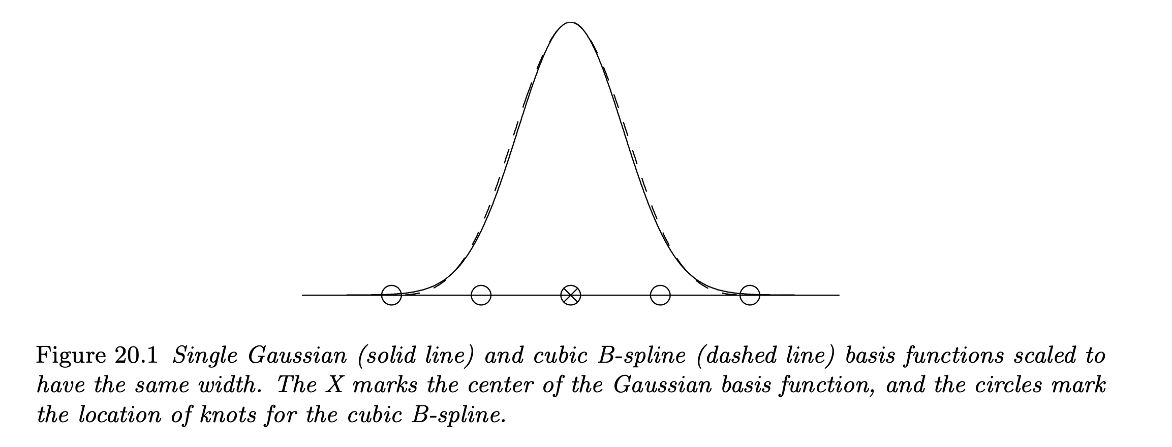
• An example of approximating the normal curve by the cubic B-spline basis functions:

 

• B-splines have a more complex functional form than Gaussian radial basis functions, but has compact support which leads to sparser design matrix. This can be exploited for enhancing computational efficiencies.

• Gaussian radial basis function usually produces smoother functions than B-spline as they are infinitely differentiable in the support.

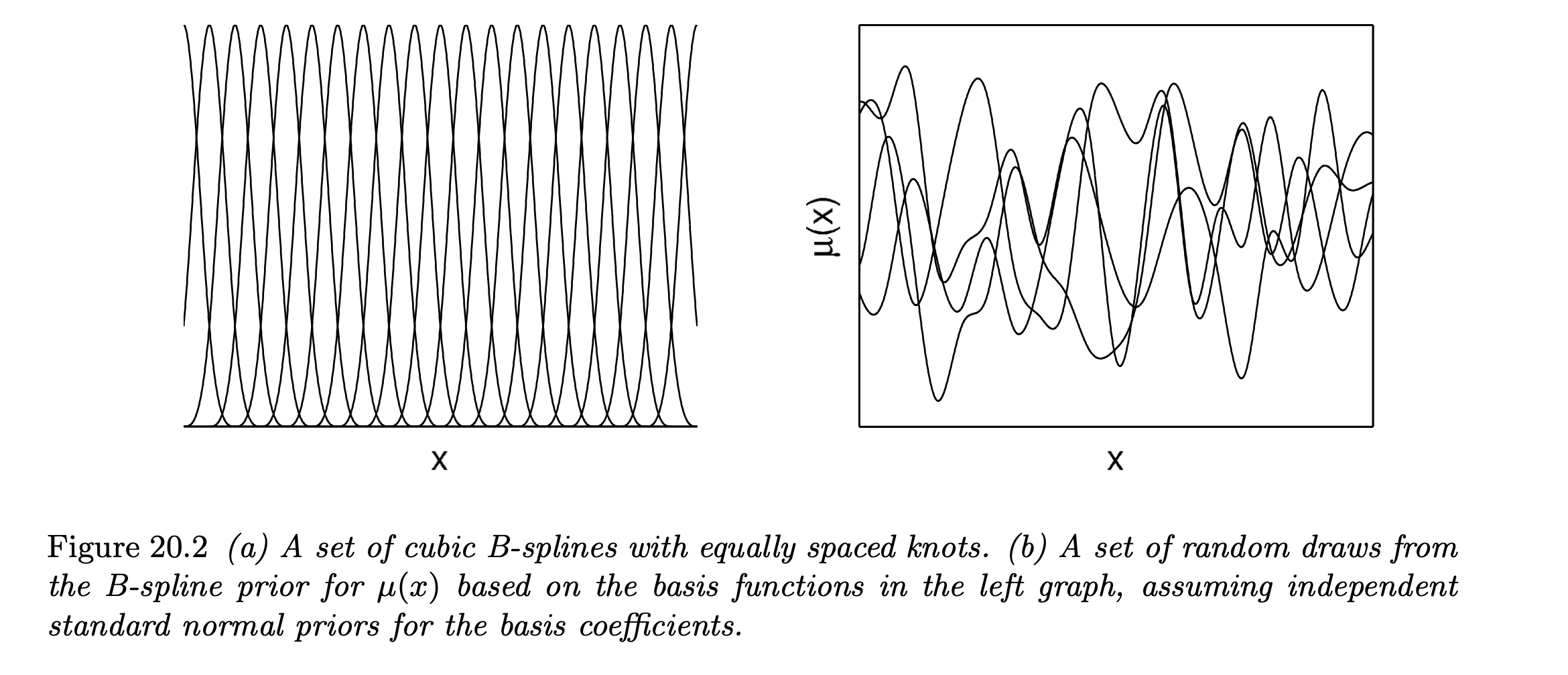
• An example of 4 realizations of prior for a nonparametric function using the cubic B-spline basis functions:

 

• Note that the number of basis functions (splines) $H$ directly impacts the flexibility of the resulting approximation of a target function.
• In this setting, our model is conditionally linear on the selected basis functions and we can apply the model fitting ideas of standard linear regression like the Least Squares method to estimate the basis coefficients $\beta$.

$$ \begin{aligned} y_i = \mu(x_i) + \epsilon_i = w_i\beta +\epsilon_i, \quad w_i = (b_1(x_i), b_2(x_i), \dots, b_H(x_i)) \end{aligned} $$

 

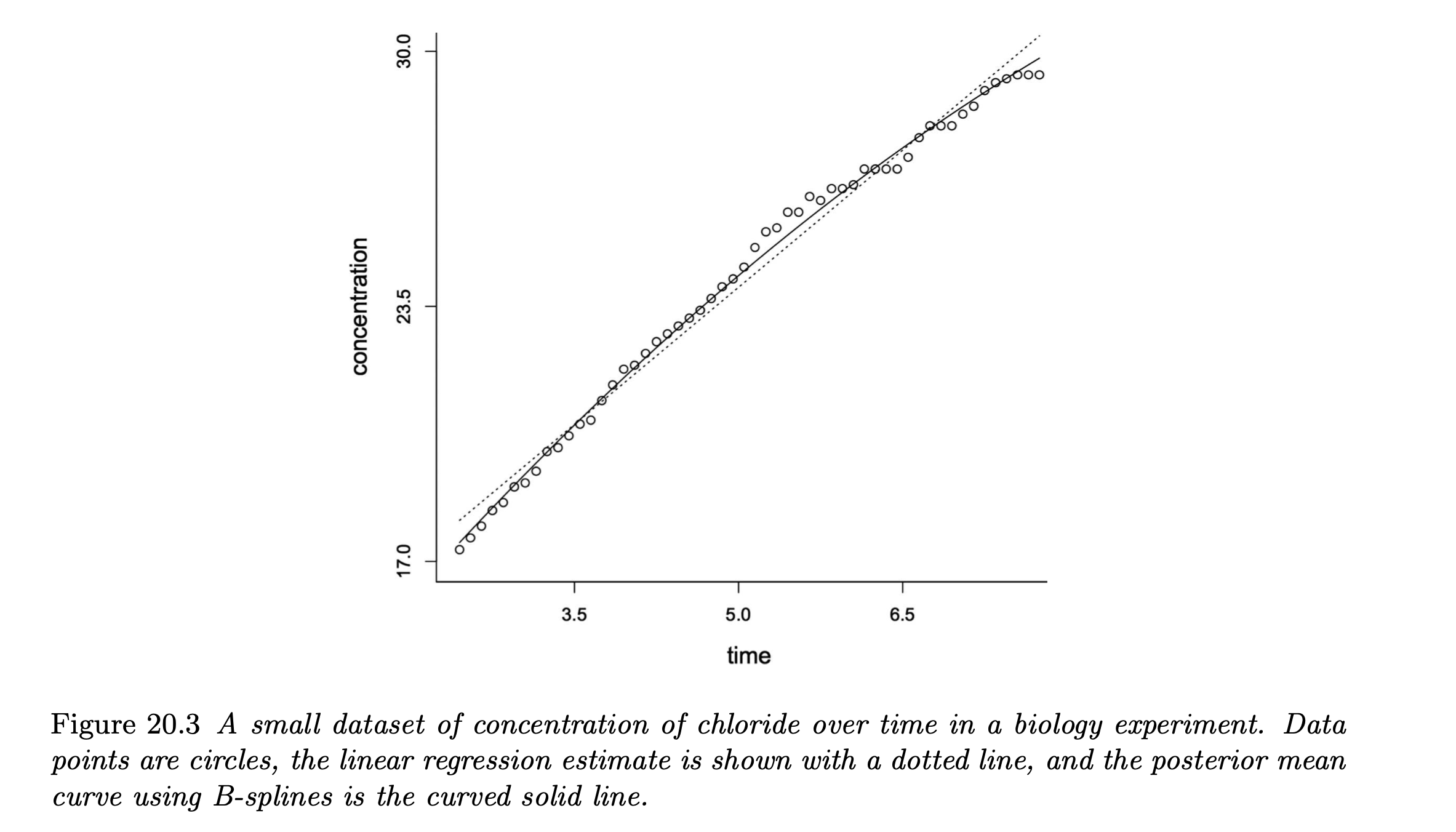
• An example of estimating the nonlinear curve by B-splines:

 

• Note that the posterior mean curve is attained by averaging over the posterior distributions of the basis coefficients for each of the basis functions.

 

Deciding number of knots for B-splines

In applying splines, we need to specify the number of knots and their locations.

• The most naive approach is to arbitrarily choose sufficient number of knots (no optimization).
• As a Bayesian alternative, we can set priors on the number and locations of each knots which is called as a free knot approach. However, this idea faces computational challenges as it requires highly efficient reversible jump MCMC (between 0/1) for posterior computation.
• Rather, we can select sufficiently many knots and implement variable selection to shrink the coefficients of the less important splines to near zero. This can be done by introducing a shrinkage prior that is concentrated near zero with heavy tails.

 

---

20.2 Basis selection and shrinkage of coefficients

 

Let’s take a closer look at the basis selection by focusing on the single-predictor nonparametric regression model with Gaussian residuals.

$$ \begin{aligned} y_i \sim N(w_i\beta, \sigma^2), \quad &w_i = (b_1(x_i), \dots, b_H(x_i)) \\[10pt] &b = \{ b_h \}_{h=1}^H \text{ denote a prespecified collection of potential basis functions} \end{aligned} $$

 

• In practice, we are mostly uncertain in which basis functions are really needed.

 

To allow less important basis functions to naturally be excluded from the model, we introduce an auxilary variable $\gamma$ to denote model index such that:

$$ \begin{aligned} &\gamma = (\gamma_1, \dots, \gamma_H) \in \Gamma \\[10pt] &\begin{equation} \gamma_h= \begin{cases} 1, & \text{basis function }b_h \text{ should be included}\ \\ 0, & \text{otherwise} \end{cases} \end{equation} \end{aligned} $$

 

• $\Gamma$ is a model space containing $2^H$ possibilities for $\gamma$’s.

 

For a complete Bayesian model specification, we require a prior over the model space $\Gamma$ as well as a prior for the non-zero basis coefficients $\beta_\gamma = \{ \beta_h: \gamma_h = 1 \}$.

• A simple specification is by using the mixture prior such that:

$$ \begin{aligned} \beta_h &\sim \pi_h \delta_0 + (1-\pi_h)N(0, \kappa_h^{-1}\sigma^2) \quad (\delta_0 \text{ is a degenerate distribution}) \\[10pt] \pi_h&\sim Beta(a_h, b_h)\\ \sigma^2 &\sim \text{Inv-}\Gamma(a,b) \\ \kappa_h &\sim \Gamma(0.5, 0.5) \quad (\text{to induce a heavy-tailed Cauchy prior for }\beta's) \\[15pt] \Rightarrow \gamma_h &\sim Bernoulli(1-\pi_h) \end{aligned} $$

 

• Hence, each of the basis coefficients will be set to 0 with probability $\pi_h$ (unimportant basis functions) and drawn from the Normal prior otherwise (important basis functions).
• In this prior specification, the joint posterior density for $\gamma$ can be tracked analytically using conjugacy, but the posterior probability for a specific model $\gamma_h$ is intractable since it requires averaging over all potential candidates of $\gamma$ ($2^H$).

• So we must use approximation such as MCMC-based stochastic search algorithm to identify high posterior probability models in the model space, or Gibbs sampling to iteratively updates $\gamma_h$ from its Bernoulli full conditional posterior.

• Anyways, the key takeaway is that we can potentially conduct model selection to obtain a simplified model without the unnecessary basis functions by averaging the joint posterior $p(y|X, \gamma)$ with respect to $\gamma$.

 

One possible drawback of this Bayesian variable selection for basis functions is that it might be sensitive to the initial choices of basis functions.

• We can potentially include multiple types of basis functions and implement Bayesian variable selection to find out the subset of basis functions doing the best job at parsimoniously characterizing the curve.
• So whenever possible, prior information should strongly inform the selection of basis functions.

 

Shrinkage priors

The basis selection method by introducing an auxilary model index variable $\gamma$ is indeed appealing, but it comes with a computational price.

• Since the number of possible models to consider is $2^H$, for sufficiently large number of basis functions, only a small percentage of the whole model space will be visited by our MCMC sampleers even in several hundreds of thousands of iterations.
• This gets even worse for non-conjugate priors.

 

One possible remedy for this problem is to use shrinkage priors for the coefficients, where the basis coefficients are avoided from being set exactly to zero.

• An appropriate prior for this purpose should have high density at zero, while having heavy tails to avoid over-shrinking the signals of important basis functions.
• The most useful shrinkage priors can be expressed as scale mixtures of Gaussians as follows:

$$ \begin{aligned} \beta_h &\sim N(0, \sigma_h^2), \\[10pt] \sigma^2_h &\sim G, \quad (G\text{: gaussian mixtures for the variances}) \end{aligned} $$

 

• For choice of the mixture distribution G, we can use several priors such as the Cauchy prior, Laplace (double exponential) prior or the generalized double Pareto prior.

 

According to the author, the generalized double Pareto prior is specifically mentioned that this distribution can indirectly be sampled by reparamerization of its parameters using Normal, Exponential and Gamma distributions.

$$ \begin{aligned} gdP(\beta|\;\xi,\alpha) &= \frac{1}{2\xi}\Big( 1 + \frac{\lvert \beta \rvert}{\alpha\xi}\Big)^{-(\alpha+1)}, \quad (\xi >0, \alpha>0 \text{ are scale and shape parameters}) \\[10pt] &\Leftrightarrow \\[10pt] \beta &\sim N(0, \sigma^2) \\[5pt] \sigma &\sim Exp(\lambda^2/2)\\[5pt] \lambda &\sim \Gamma(\alpha,\eta) \\[5pt] \xi &= \eta/\alpha, \quad (\text{typically, }\alpha = \eta =1) \end{aligned} $$

 

• We can use a simple Gibbs sampler to get posterior samples for each of the parameters and basis coefficients (for more detail refer p.494).
• We expect from this generalized double Pareto shrinkage prior to shrink many of the basis coefficients towards zero, while not shrinking the coefficients for the more important bases much at all in high-dimensional settings.

 

---

20.3 Non-normal models and multivariate regression surfaces

 

Non-normal models

We can relax our model to accommodate heavier-tailed residual densities which can handle possible outliers by using a scale mixture of the gaussians.

• One example is the “inverse-gamma scale mixture of normals representation” of the residual density such that:

$$ \begin{aligned} y_i \sim N(\mu(x_i), \phi_i\sigma^2), \quad \phi_i\sim \text{Inv-}\Gamma(\nu/2, \nu,2) \end{aligned} $$

 

• Each response has different variance structure and the value of $\phi_i$ will control the scale of the response, downweighting the influence of outliers on the posterior distribution of $\mu(x)$.
• To extend the response distribution to the exponential families, we can use various link functions just like for the GLMs in the same framework as above.

 

Multivariate regression surfaces

So far, we have focused on regression models with a single predictor. What can we do to incorporate multiple predictors?

For multivariate cases, the curse of dimensionality arises.

• Computational methods that work for small number of predictors may not scale well as predictors are added. This is because the number of basis functions needed increase exponentially with respect to increase in the predictor variables.
• We need sufficiently large number of data points, prior information or some restrictions to reliably estimate a nonparametrical multivariate regression because the observations are sparsely distributed in high dimensional predictor surfaces.
• To account for this, a commonly used assumption is the additivity of the curve function by univariate regression functions:

$$ \begin{aligned} \mu(x) &= \mu_0 + \sum_{j=1}^p \beta_j (x_j) \\[10pt] \beta_j(x_j) &= \sum_{h=1}^{H_j}\theta_{jh}b_{jh}(x_j) \end{aligned} $$

 

• Above, an unknown coefficient function for each of the predictor $\beta_j()$ is expressed as a linear combination of a prespecified set of basis functions $b_j = \{b_{jh} \}_{h=1}^{H_j}$.

• Additivity assumption might not be plausible when there is interaction effect among the predictor variables. In this case, we can think of using tensor product specification (for more detail refer p.497).

• In addition to additivity assumptions, we can set constraint on shape of the priors to further enhance the efficiency.
• For example, if we are certain that our response is nondecreasing in some of the predictors, we can set nondecreasing constraint on certain $\beta_j(x_j)$ in the additive expansion. Let’s check this by an example.

 

Example. A nonparametric regression function that is constrained to be nondecreasing

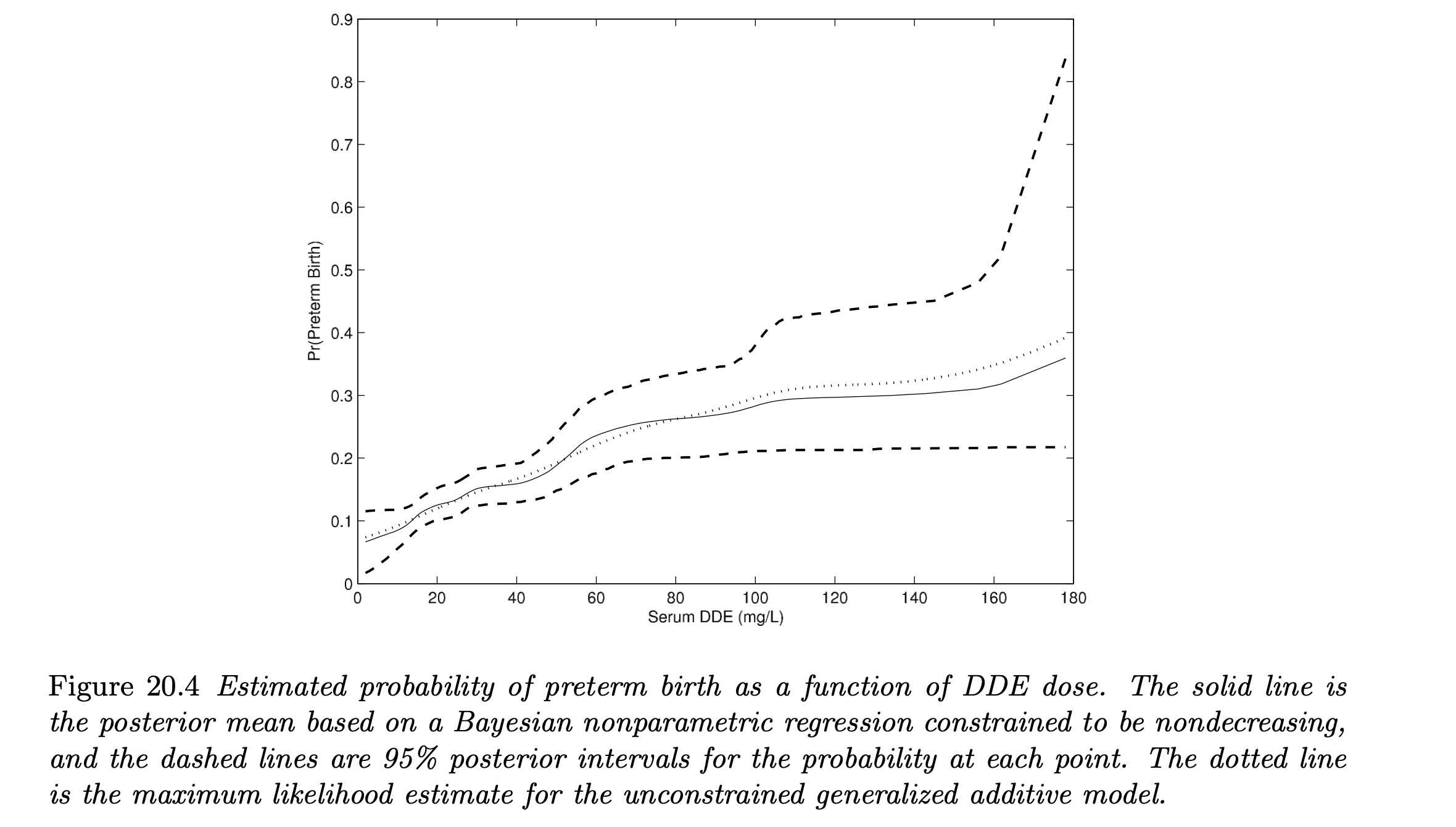
We consider an example of pregnant women data in the U.S. Collaborative Perinatal Project, where the incidence of “preterm birth” is studied in relationship with 5 different covariates (cholesterol, triglyceride level, age, BMI, smoking status) and “DDE concentration” (DDE is a persistent metabolite of the pesticide DDT).

Let’s see how we can incorporate a nondecreasing constraint on the regression function relating level of DDE to the probability of preterm birth.

• This constraint is made because we have a reasonable “a-priori belief” that covariate-adjusted premature delivery risk is nondecreasing in dose of DDE.

 

We use semiparametric probit additive model such that:

$$ \begin{aligned} Pr(y_i=1|\theta, x_i, z_i) &= \Phi\Big( \alpha_0 + \sum_{k=1}^5z_{ik}\alpha_k + f(x_i)\Big) = \Phi\big(z_i\alpha + f(x_i) \big) \\[10pt] &(z_i:\text{covariate variable}, \;x_i:\text{DDE level}, \;y_i:\text{indicator of preterm birth}) \end{aligned} $$

 

• The covariate adjustments are parametric (although not described), while $f(x)$ is characterized nonparametrically as a nondecreasing curve using splines with a carefully structured prior on the basis coefficients. The basis functions are simply piecewise linear functions with a dense set of knots.

• To incorporate the constraint, we choose a prior for the basis coefficients that does not allow negative values. Since these coefficients are directly the slopes of the regression lines at each knots, the resulting nonparametric curve cannot be decreasing.

• For the (latent) basis coefficients, we use first-order normal random walk autoregressive prior such that:

$$ \begin{aligned} \beta_j^* &\sim N(\beta_{j-1}^*, \;\sigma_\beta^2) \\[10pt] \sigma_\beta^2 &\sim \text{Inv-}\Gamma(a, b), \quad (a,b \text{ are some constants})\\[10pt] \beta_j &= \textbf{1}\{\beta_j \geq \delta \}\beta_j^*, \quad \delta \sim \Gamma(c, d) \quad (c,d \text{ are some constants}) \end{aligned} $$

 

• Note that $\delta$ is a positive threshold parameter which links latent $\beta_j^*$ to the slopes $\beta_j$.
• By implementing an MCMC algorithm for posterior computation, we get the following estimated curve $f(x)$:

 

---

References

• Gelman et. al. 2013. Bayesian Data Analysis. 3rd ed. CRC Press. p.487-498.