[Bayesian Statistics] Gaussian Process Models (1)

2021, Nov 15

Ch 21. Gaussian Process Models

This post is a summary of Chapter 21 of the textbook Bayesian Data Analysis.

In the previous chapter, we considered basis function expansions to approximate nonlinear structure of the response function.

Specifically, we used a set of knots on a prespecified grid, where the linear combination of basis functions on those grids led to reasonable approximation of our target function if appropriate knots were chosen. Moreover, we made use of shrinkage priors to effectively discard those knots that are insignificant.

While this approach is indeed plausible, it can sometimes be inefficient in that there exists some computational burden for the high-dimensional set of knots and that there may nonetheless be some sensitivity to the initial choice of knots.

Hence in this chapter, we are going to take a look at the Gaussian Process as a prior distribution for the regression function, which is a flexible class of models that produces marginal Gaussian distributions for all of its finite-dimensional subspaces. It has some noticeable computational and theoretical advantages we can possibly exploit in the model structure.

21.1 Gaussian process regression

21.2 Example: birthdays and birthdates

21.1 Gaussian process regression

In a nutshell, Gaussian process can be thought of as an infinite-dimensional generalization of the Gaussian (Normal) distribution.

The realizations from a Gaussian process is nonlinear functions, thus it can naturally be used as a prior distribution for an unknown nonlinear regression function which we will denote as $\mu(x)$. Now, we don’t have to explicitly specify basis functions!

We denote a Gaussian process prior as $\mu \sim GP(m, k)$, where the $n$ number of random values at the prespecified points $x_1, \dots, x_n$ are generated by $n$ x $1$ mean vector $m(\textbf x)$, and $n$ x $n$ covariance matrix $K$.

$$ \begin{aligned} \mu(x_1), \dots, \mu(x_n) \sim N\Big(m(\textbf x), \;K\big(x_1, \dots, x_n\big) \Big) \end{aligned} $$

Without the points $x_1, \dots, x_n$ being specified, $m$ is a continuous mean function and $k$ is the corresponding covariance function.
Thus, the mean and covariance function $m, K$ are the key components sufficient for fully characterizing a Gaussian process, thus we need to take a closer look at each of them.

Mean function

Since there are infinitely many parameters characterizing the mean function $m$, it is typically centered (approximated) by a linear model such that $m(x) \equiv X\beta$.
We can choose hyper priors for the coefficients $\beta$ just as we did in the previous chapters.
This “Centering of the Gaussian process on a linear model” addresses curse of dimensionality as well as it can useful for interpolating across the unobserved data regions.

Covariance function

This function $k$ specifies the covariance structure between the process of any given two points $x$ and $x^\prime$.
For a prespecified $n$ number of data points $x_1, \dots, x_n$ , $K$ is a $n$ x $n$ covariance matrix with element $(p, q)$ corresponding to $k(x_p, x_q)$ for which the book uses the shorthand notation $k(x, x^\prime)$.
It controls the smoothness of the realizations from the Gaussian process and the degree of shrinkage towards the mean.
There are various covariance functions with respect to the domain of application. For example, the Matérn covariance function is often used in spatial data domain.
In this chapter, the squared exponential covariance function is mostly used.

$$ k(x, x^\prime) = \tau^2 exp\Big( -\frac{\lvert x - x^\prime \rvert^2}{l^2} \Big) $$

For other types of covariance functions, refer wikipedia.
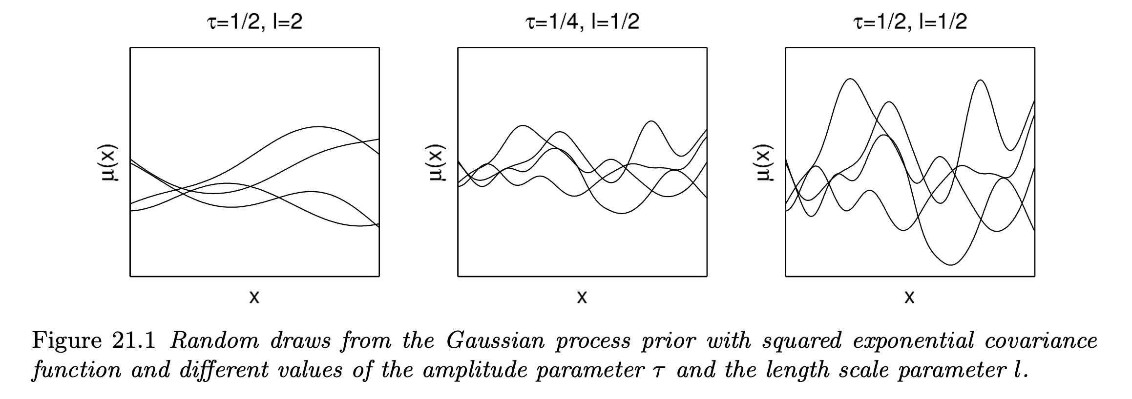
In terms of the exponential covariance function, large $\tau$ means there are more ups and downs in the process, whereas for large $l$ the process is more smoothed (less dependency).

One appealing advantages of using Gaussian process priors is that we can fit a wide range of smooth surfaces while being computationally tractable even for sufficiently large number of predictors (high-dimensional regression space).

In fact, Gaussian processes with typical covariance functions are actually equivalent to infinite basis expansions.

For instance, let’s consider a case for $n$-dimensional regression functions such that:

$$ \begin{aligned} \mu(x) &\equiv \sum_{h=1}^H \beta_h b_h(x), \quad \beta = (\beta_1, \dots, \beta_H) \sim N_H(\beta_0, \Sigma_\beta) \\[10pt] &\Rightarrow \big(\mu(x_1) ,\dots , \mu(x_n) \big) \sim GP_n\Big( \big(m(x_1), \dots, m(x_n) \big), \; K \Big) \\[10pt] &\text{where } \;m(x) = b(x)\beta_0, \quad k(x, x^\prime) = b(x)^T \Sigma_\beta \;b(x^\prime), \quad b(x) = \big( b_1(x), \dots, b_H(x) \big)^T \end{aligned} $$

Here, an arbitrary regression surface on a $n$-dimensional space ($n$ number of predictor variables) is approximated by a Gaussian process whose parameter structure is again modeled as an expansion of $H$ basis functions in the marginal subspaces.

Note that we can add structural prior assumptions such as smoothness, nonstationarity, periodicity and hierarchical structures to our model by the choice of adequate covariance functions. Moreover, the additive property of normal distributions makes it easy to combine different covariance functions.

Inference for unobserved data points

Given a Normal likelihood for the observation $y_i \sim N(\mu_i, \sigma^2)$, we can analytically derive the conditional posterior distribution for the mean vector $\mu$. In practice, our main concern is often in the interpolation for the unobserved data points $\tilde x$ with the corresponding mean vector $\tilde \mu$.

Then, given Gaussian process prior $GP(0, k)$, the joint density for observations $y$ and $\tilde \mu$ at unobserved locations $\tilde x$ is simply another multivariate normal such that:

$$ \begin{pmatrix} y \\ \tilde \mu \end{pmatrix} \sim N\Big( \begin{pmatrix} 0 \\ 0 \end{pmatrix}, \begin{pmatrix} K(x,x) + \sigma^2I & K(\tilde x, x) \\ K(x, \tilde x) & K(\tilde x, \tilde x) \end{pmatrix} \Big) $$

Then, by the property of multivariate normal distribution, the conditional posterior of $\tilde \mu$ given all other hyper parameters $\tau, l, \sigma$ (assume squared exponential covariance function) is obtained as a normal distribution with the following parameters:

$$ \begin{aligned} \tilde \mu | x, y, \tau, l, \sigma &\sim N(E[\tilde \mu], cov(\tilde \mu)) \\[10pt] E[\tilde \mu] &= K(\tilde x, x)\big( K(x,x) + \sigma^2I \big)^{-1}y \\[5pt] Cov(\tilde \mu) &= K(\tilde x, \tilde x) - K(\tilde x, x) \big( K(x,x) + \sigma^2I \big)^{-1}K(x,\tilde x) \end{aligned} $$

One might possibly think that we can easily get the interpolated estimates for the unobserved data points $\tilde x$ by the above formula, but there exists one huge problem.

We can see that the computation involves matrix inversion of $\big( K(x,x) + \sigma^2I \big)^{-1}$, which requires $O(n^3)$ computational complexity. Since this calculation for every data points has to be repeated for every iteration of MCMC sampler, the computation expense increases so rapidly with just a few thousand data points and few hyper parameters. For example, if we have 1000 observations with 3 hyperparameters and 10 number of predictor variables, the matrix is of dimension 30000 x 30000. and we need to calculate the inverse of this.

Thus in terms of practicality, the covariance function is often approximated by some statistical methodologies.

One possible way of approximation is by using Markov Random Field, which is basically assuming conditional independence on the observations so that the covariance matrix becomes sparse (most of its elements are zero). With additional assumption of additivity (as discussed in Ch.20) in the latent function, this approach can significantly reduce computational complexity to about $O(n) \sim O(n^{3/2})$.
For the case when the length scale of dependency in the latent function is relatively long (function is smooth), we can consider using reduced rank approximations such as PCA for the covariance matrices. The resulting computational complexity is around $O(mn^2)$ with $m$ « $n$.

Marginal likelihood and posterior

Similary, by utilizing the convenient property of multivariate normal distributions, we can analytically derive the (log) marginal posterior distributions for the parameters.

Let’s again consider a normal likelihood for the observation. Then from the joint density of $y$ and $\mu$, we can integrate out the $\mu$ to get the log marginal likelihood given the hyper parameters such that:

$$ log p(y|\tau, l, \sigma^2) = -\frac{n}{2}log(2\pi) - \frac{1}{2}log\lvert K(x,x) + \sigma^2I \rvert - \frac{1}{2} y^T \big( K(x,x) + \sigma^2I\big)^{-1}y $$

From this, we can just multiply the priors distributions for the hyper parameters to get the unnormalized marginal log posteriors for any specific hyper parameters $\tau, l, \sigma^2$. For example, if we are interested in the log posterior of $\tau$ (assume hyper parameters are independent), then we can analytically calculate the following formula:

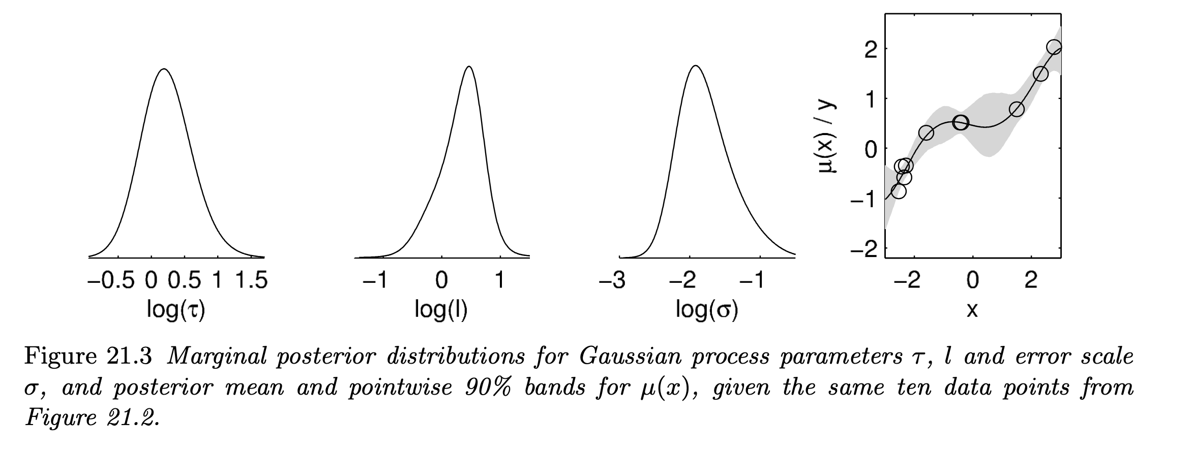
$$ \log(\tau) \propto \int\int\int log p(y|\tau, l, \sigma^2) p(\tau) p(l) p(\sigma^2) \;dy\;dl\;d\sigma^2 $$

In this sense, the posteriors derived for $\tau, l \sim t_4^+(0,1)$ and $\sigma \sim log \; Unif$ are:

21.2 Example: birthdays and birthdates

Now we will take a look at a specific example of how Gaussian processes are used as components in a large model.

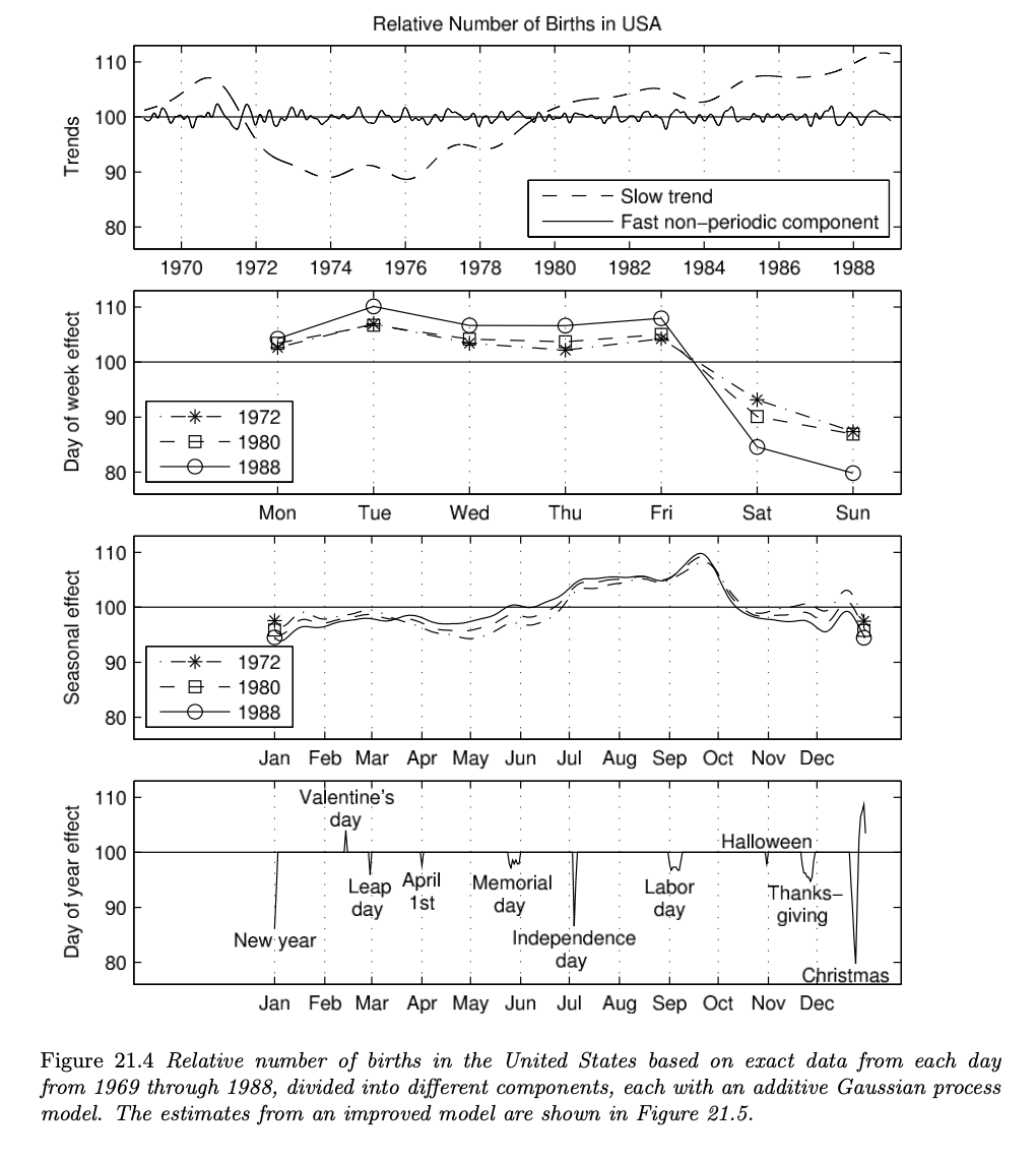
The illustrated example is the analysis of patterns in birthday frequencies in the United States from 1969 to 1988.
A pilot study indicates that there is a tendency of relatively fewer births on Halloween and more births on Valentine’s Day.
Regarding this, the analysis was made to infer about the underlying birth tendency with respect to special days throughout an year, along with the day-of-week effect, seasonal pattern effect and long-term effect.

The overall model is an additive time-series model, which is decomposed into 6 different submodels.

$$ y_t(t) = f_1(t) + f_2(t) + f_3(t) + f_4(t) + f_5(t) + \epsilon_t, \quad (t\text{ is time in days}) $$

1. Long-term trend model

modeled by a Gaussian process with squared exponential covariance function such that:
$$ f_1(t) \sim GP(0, k_1), \quad k_1(t,t^\prime) = \sigma_1^2 \;exp\Big( -\frac{|t-t^\prime|^2}{l_1^2} \Big) $$

2. Shorter-term variation model

modeled by Gaussian process with squared exponential covariance function with different amplitude and scale parameter such that:

$$ f_2(t) \sim GP(0, k_2), \quad k_2(t,t^\prime) = \sigma_2^2 \;exp\Big( -\frac{|t-t^\prime|^2}{l_2^2} \Big) $$

3. Weekly quasi-periodic pattern

modeled as a product of periodic and squared exponential covariance function such that:

$$ f_3(t) \sim GP(0, k_3), \quad k_3(t, t^\prime) = \sigma_3^2 \; exp\Big(-\frac{2sin^2(\pi(t-t^\prime)/7)}{l_{3,1}^2}\Big) \;exp\Big(-\frac{|t-t^\prime|^2}{l_{3,2}^2}\Big) $$

4. Yearly smooth seasonal pattern

modeled again as a product of periodic and squared exponential covariance function such that:

$$ f_4(t) \sim GP(0, k_4), \quad k_4(t, t^\prime) = \sigma_4^2 \; exp\Big(-\frac{2sin^2(\pi(t-t^\prime)/365.25)}{l_{4,1}^2}\Big) \;exp\Big(-\frac{|t-t^\prime|^2}{l_{4,2}^2}\Big) $$

Note that the period was set to 365.25 to match the average length of the year.

5. Special days including interaction term with weekend

concretely specified as the indicator function including “New Year’s Day”, “Valentine’s Day”, “Leap Day”, “April Fool’s Day”, “Independence Day”, “Halloween”, “Christmas” and the days between Christmas and New Year’s

$$ f_5(t) = I_{\text{special day}}(t) \beta_a + I_{\text{weekend}}(t) I_{\text{special day}}(t)\beta_b $$

$I_{\text{special day}}(t)$ is a row vector of 13 indicator variables corresponding to each of the special days (one-hot encoded).
$I_{\text{weekend}}(t)$ is an indicator variable that returns 1 if $t$ is Saturday or Sunday and 0 otherwise.
The corresponding coefficients $\beta_a, \beta_b$ are vectors of length 13.

6. Unstructured errors

$$ \epsilon_t \sim N(0,\sigma^2) $$

For the hyperparameters of this model, weakly informative log-t priors were set for the time-scale parameters $l$, and log-uniform priors for the rest of the hyperparameters. The daily birth counts were normalized using Z-transformation.

Furthermore, the joint covariance function was assumed to have additivity, thus the covariance function for the sum is decomposed into the sum of marginal covariance functions.

$$ k(t,t^\prime) = k_1(t,t^\prime) + k_2(t,t^\prime) + k_3(t,t^\prime) + k_4(t,t^\prime) + k_5(t,t^\prime) $$

The marginal posteriors were derived analytically by the marginal posterior calculation illustrated above. We can of course use MCMC samplers, but it would be slow due to $n$ = 20 x 365.25 number of data points.

The book also introduces an improved model, with the modification being made by adding a “very short time-scale non-periodic component” to explain special effects for each day of the year and also the refinement of the leap day. Overall structure of the model is quite similar as the initial model, so the details are omitted here. If interested, refer p.507 - p.510.

In summary, the key takeaway from this example is that by using Gaussian process priors, we can flexibly account for different scales of variation for different components in the model.

References

Gelman et. al. 2013. Bayesian Data Analysis. 3rd ed. CRC Press. p.487-498.

# bayesian-statistics # gaussian-process

[Bayesian Statistics] Gaussian Process Models (1)

Ch 21. Gaussian Process Models