[Bayesian Statistics] Gaussian Process Models (2)

2021, Nov 29

 

Ch 21. Gaussian Process Models (cont’d)

The contents of this post is subsequent to this post.

---

Table of Contents

21.3 Latent Gaussian process models

21.4 Functional data analysis

21.5 Density estimation and regression

 

---

21.3. Latent Gaussian process models

So far, we talked about using Gaussian process as a prior for an arbitrary function. In this setting, we implicitly assumed that the likelihood \(p(y | \theta)\) is normal. This wasn’t a huge deal for any type of continuous data, as transformation technics are available for such cases to make them approximately normal.

However, we now focus on non-Gaussian likelihoods where such assumptions are violated. For instance, how can we put a prior to an indicator function where the outcomes are binary? or some function that returns discrete data like counts?

In this situation, we can define a latent function $f$ which through a link function determines the likelihood \(p(y | f, \phi)\) , and set Gaussian process prior on that latent function (just like in the GLMs).

Then the conditional posterior density of the latent $f$ is \(p(f|x,y,\theta,\phi) \propto p(y|f,\phi)p(f|x,\theta)\) , which is proportional to the likelihood times the prior of the latent function, which we will assume to be a Gaussian process.

The textbook mentions that we can use GP-specific samplers for extracting the posterior samples from this model specification, or we can approximate the posterior (of the latent function $f$) by using the normal approximation.

 

$$ \begin{aligned} \Rightarrow p&(f | x,y,\theta, \phi) \approx N(f |\hat f, \Sigma) \\[10pt] \text{where }&\hat f \text{ is the posterior mode}, \\ &\Sigma^{-1} = K(x, x) + W, \\ & K(x,x) \text{ is the prior covariance matrix,} \\ & W = diag(w_{ii}), w_{ii} = \frac{d^2}{df^2} log p(y | f_i, \phi)|_{f_i = \hat f_i} \end{aligned} $$

 

• the posterior mode $\hat f$ can be derived using the variational inference or expectation propagation.

 

Example. Leukemia survival times

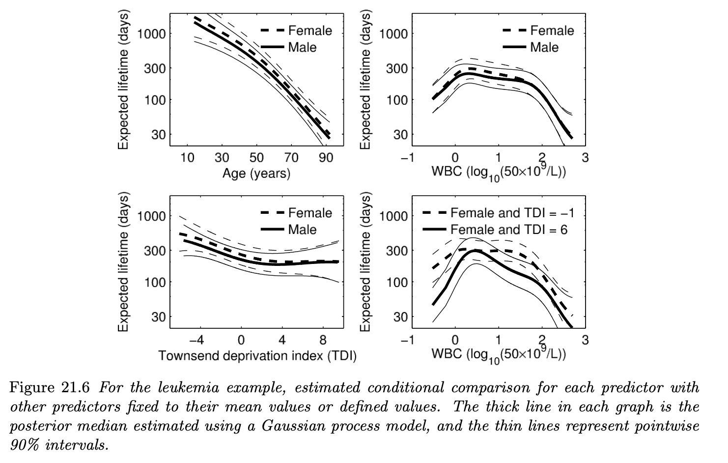
As an illustration of a Gaussian process model with non-Gaussian data, the book introduces analysis of the survival time of leukemia in adults. The predictor variables were age, sex, WBC (white blood cell count) and Townsend score (detail is omitted) and the response was the survival time with its censoring indicator $z$ of 0/1.

Since the response is dependent on the binary indicator variable, they have used log-logistic model. The likelihood for the reported number of leukimia cases for each subjects is:

 

$$ \begin{aligned} p(y | -) &= \prod_{i=1}^n \Big( \frac{ry^{r-1}}{exp(f(X_i))} \Big)^{1-z_i} \Big( 1 + (\frac{y}{exp(f(X_i))})^r \Big)^{z_i-2}, \\[5pt] &f_i(X_i) = \alpha + X_i\beta + \mu(X_i) \end{aligned} $$

 

where $r$ is the shape parameter and $z_i$ is the censoring indicator for subject $i$.

In this model specification, we set Gaussian process prior with exponential covariance function on the $\mu$, which fully defines the latent function $f$. Furthermore, for a complete Bayesian inference, weakly informative priors were set for the hyper parameters.

To derive the posteriors for each of the parameter components, numerical approximation technics such as the Laplace’s method and CCD integration was used. Figure 21.6 shows the estimated conditional comparison of each predictor with all other predictors fixed to certain values.

 

 

If we take a look at the bottom right figure, we can see that the predictor WBC has interation with Townsend score (TDI). Since concrete definition of each of the predictor variables was not provided in the textbook, I will not dig further into the interpretation of their interation effects. However, the key takeaway is that the Gaussian process prior on the function $\mu$ was able to account for the interaction effects of the predictors.

---

21.4 Functional data analysis

This section briefly introduces the idea of functional data analysis.

The main idea is that now we are considering the responses and predictors for a subject as a random functions defined at infinitely many locations, rather than vector-valued random variables.

As an example, suppose we have an observation $y_{ij}$ collected at a point $t_{ij}$. With some possible uncertainty, we can model the observations as

 

$$ y_{ij} \sim N\big( f_i(t_{ij}), \sigma^2 \big) $$

 

Now the mean structure of this normal distribution is a function, not a scalar. Furthermore, suppose we want to incorporate covariates $x_i$ for each subjects in the mean structure $f$. In this situation, Gaussian process can be used as a prior for this functional relationship.

For example, the ordinary regression can be expressed as:

 

$$ \begin{aligned} y_{ij} &\sim N( f(x_i, t_{ij}), \sigma^2), \\[10pt] f &\sim GP(m, k), \quad (k\text{ is expanded to include additional dimension of }t) \end{aligned} $$

 

For example, we can use the exponential covariance function for $k$ such that

 

$$ k = \tau^2\Big( -\big( \sum_{j=1}^p \frac{(x_j - x_j^\prime)^2}{l_j^2} + \frac{(t-t^\prime)^2}{l_{p+1}^2} \big) \Big) $$

 

Again, the main point is that the Gaussian process is used as a prior for a “function”.

 

---

21.5 Density estimation and regression

The discussions until now have focused on how we can use Gaussian process as a prior for a functional component in a model.

Now, we shift our attention to nonparametrically modeling the likelihood using Gaussian process. There are several ways to do this where one of the most famous method is by the Dirichlet process (to be addressed in subsequent chapters), but in this section the logistic Gaussian process (LGP) is introduced.

 

Density estimation

As a simple example, suppose we are interested in modeling the one-dimensional likelihood under i.i.d. assumptions (i.e. $y_i \overset{iid}{\sim} p$).

For estimating the likelihood of the given observations $\textbf y$, the LGP first generates an arbitrary random surface (in this case, a curve) from a Gaussian process and transforms this surface to fit to the observations. Then the kernel likelihood is divided by its integration over the whole parameter space to make it satisfy probability distribution:

 

$$ p(y|f) = \frac{e^{f(y)}}{\int e^{f(y^\prime)}dy^\prime }, \quad f\sim GP(m,k) $$

 

• The parameter functions for the Gaussian process $m, k$ are defined as usual.

One huge challenge left unsolved is the integral at the denominator, as it requires integration of a continuous function $f$. Since it cannot be derived analytically in most of the situations, inference for $f$ and model parameters $m, k$ are usually done by MCMC methods.

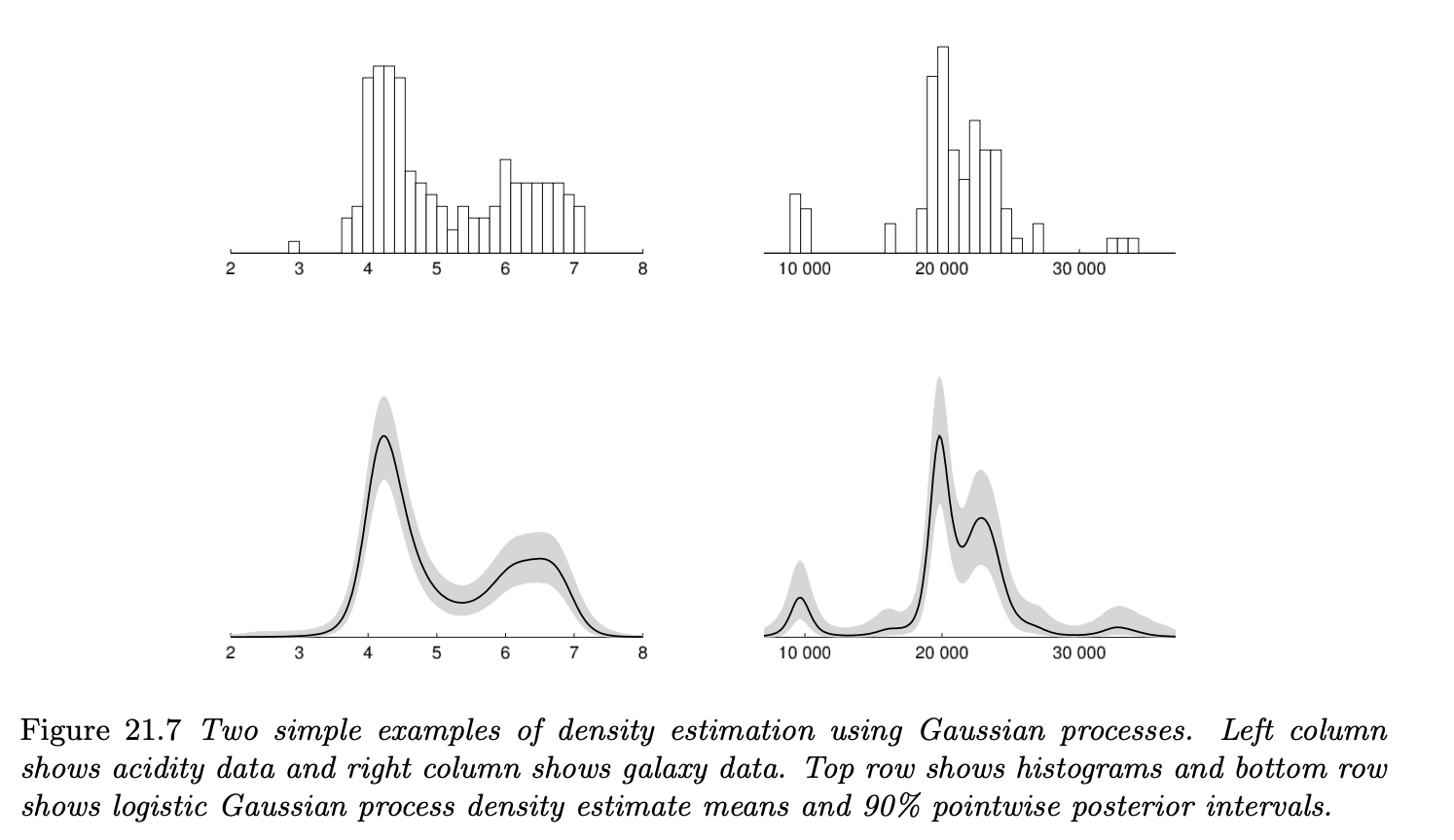
Figure 21.7 illustrates the estimated densities from data using Gaussian processes. We can see that the estimated density is multimodal, which reasonably corresponds to the observed histogram.

 

 

Density regression

We can extend the above LGP prior to include covariates (predictor variables) $\textbf x$ such that:

 

$$ p(y | x, f) = \frac{e^{f(x,y)}}{\int e^{f(x, y^\prime)}dy^\prime} $$

 

where again, $f$ is drawn from a Gaussian process $GP(m, k)$ with prespecified covariance function. One choice of such $k$ is the squared exponential covariance kernel such that:

 

$$ k\big( (x,y), (x^\prime, y^\prime) \big) = \tau^2 exp\Big( -\big( \sum_{j=1}^p \frac{(x_j - x_j^\prime)^2}{l_j} + \frac{(y-y^\prime)^2}{l_{p+1}} \big) \Big) $$

 

the hyperpriors for $l_j$ can be chosen adequately to allow variable selection for the predictors as we did in previous chapters.

Similar to the unconditional density estimation, the inference can be done by MCMC. However, computational costs can be an issue when we include multiple predictors, as each predictor adds another $p$ dimensions to the integration at the denominator.

 

Latent-variable regression

The foremost problem of posterior inference for the likelihood using the LGP was that it required the integration of the continuous density $f$ over the parameter space, which is intractable for most cases.

A simple alternative can possibly be done by including a latent variable $u \sim Unif(0,1)$ for drawing the posterior samples for the likelihood given the observations.

Suppose we are interested in estimating the posterior likelihood (density) given a one-dimensional i.i.d. observations without any predictors. The latent-variable density estimation model can be defined as the following:

 

$$ y_i \sim N\big( \mu(u_i), \sigma^2 \big), \quad u_i \sim Unif(0,1) $$

 

In this situation, we can set Gaussian process prior centered on $\mu_0$ with a squared covariance function $k$ for the mean function $\mu$.

 

$$ \mu \sim GP(\mu_0, k) $$

 

Additionally, if we can assume that the function $\mu_0$ can be approximated by a well-known density function $g_0$ for which we can analytically derive the inverse cdf $G_0^{-1}$, we can use the inverse-cdf method to extract samples from $\mu_0$.

 

$$ \begin{aligned} &\mu_0 \sim g_0\\[10pt] & \mu_0 \equiv G_0^{-1}(u_i) \quad u_i \sim Unif(0,1) \\[10pt] &\therefore \text{we have samples for }\mu_0 \\[5pt] &\Rightarrow \text{Gaussian process }GP(\mu_0, k) \text{ is completely defined!} \end{aligned} $$

 

If this is the case, we don’t have to care about the integration of $\mu$ and density estimation can be done using the property of conditionals of the multivariate Gaussian distribution by updating $\mu$ from the realized values of $u_i$.

Likewise, we can also include covariates in the above setting and then the model becomes latent-variable regression model.

 

$$ y_i \sim N\big( \mu(u_i, x_i), \sigma^2 \big), \quad u_i \sim Unif(0,1) $$

 

---

 

 

---

References

• Gelman et. al. 2013. Bayesian Data Analysis. 3rd ed. CRC Press. p.487-498.