Statistical Tests for Clinical Trials

2022, Apr 18

 

This post is an overall summary of different testing methodologies used in clinical trials.

• 1. One-Sample T-test

• 2. Two-Sample T-test

• 3. One-way ANOVA

• 4. Two-way ANOVA

• 5. Linear Regression

• 6. Analysis of Covariance

• 7. Wilcoxon Signed Rank Test

• 8. Wilcoxon Rank-Sum Test

• 9. Kruskal-Wallis Test

• 10. Binomial Test

• 11. Chi-Square Test

• 12. Fisher’s Exact Test

• 13. McNemar’s Test

• 14. Cochran-Mantel-Haenszel Test

• 15. Logistic Regression

 

---

1. One-Sample T-test

One-Sample T-test is used to infer whether an unknown population mean differs from a hypothesized value.

<Assumptions>

• i.i.d. samples from normal distribution with unknown mean μ.

<Test Setting>

 

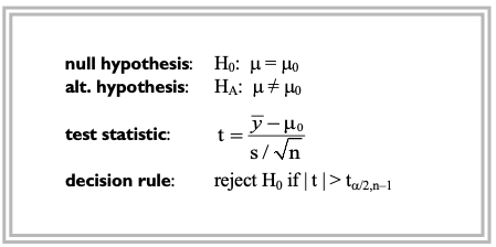
<Takeaways>

• A special case of the one-sample t-test is to determine whether a mean response changes under different experimental conditions by using “paired observations” ($\mu_d$=the mean difference, $\mu_0$= 0 , $y_i$’s = the paired-differences).
• It can be shown that the t-test is equivalent to the Z-test for infinite degrees of freedom. In other words, Z-test is equivalent to t-test in the limit of sample size. In practice, a ‘large’ sample is usually considered to be $n$ ≥ 30.
• If the assumption of normality cannot be guarenteed, the “mean” might not be the best measure of central tendency. In such cases, a non- parametric test such as the Wilcoxon signed-rank test might be more appropriate choice.
• A non-significant result does not necessarily imply that the null hypothesis is true. It only asserts insufficient evidence for contradicting the original statement.
• Statistical significance does not imply causality in observational studies, only for “randomized” controlled trials (RCT).

 

---

2. Two-sample T-test

Two-sample T-test is used to compare the means of two independent populations, denoted as $\mu_1$ and $\mu_2$.

It has ubiquitous application in the analysis of controlled clinical trials.

<Assumptions>

• The populations are normally distributed.
• Homogeneity of variance - the populations share the same variance $\sigma^2$.

<Test Setting>

 

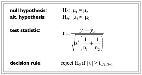
<Takeaways>

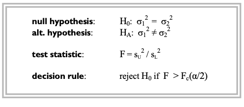
• The assumption of equal variances can be tested using the F-test:

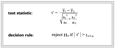
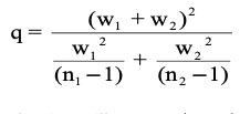
• If the assumption of equal variances is rejected, a slight modification of the t-test called as the Welch’s t-test:

• The assumption of normality can formally be checked by the Shapiro-Wilk test or the Kolmogorov-Smirnov test.
• For large enough samples, CLT (central limit theorem) holds. However, if the data is heavily skewed such that normal approximation guarenteed by CLT is not sufficiently accurate, we have to consider changing test statistic from mean to median and use Wilcoxon rank-sum test instead.

 

---

3. One-way ANOVA

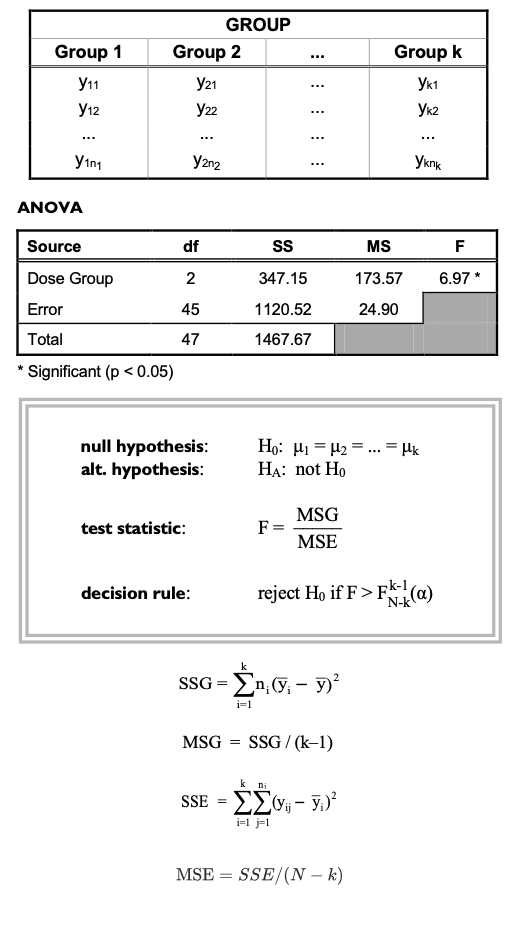
One-way ANOVA is used to simultaneously compare two or more group means based on independent samples from each group.

<Assumptions>

• normally distributed data
• samples are independent w.r.t. each group
• variance homogeneity, meaning that the within-group variance is constant across groups. This can be expressed as $\sigma_1 = \sigma_2 = \dots = \sigma_k = \sigma$

<Test Setting>

<Takeaways>

• Intuitively, if the “F statistic” that is roughly the ratio of between-group variability and within-group variability is far from 1, it is evident that the group means indeed differ.

• On the other hand, F statistic will be close to 1, if the variation among groups and the variation within groups are independent estimates of the same measurement variation, $\sigma^2$.

• In this sense, MSG is an estimate of the variability “among groups”, and MSE is an estimate of the variability “within groups”.

• The parameters associated with the F-distribution are the upper and lower degrees of freedom.

• An “ANOVA table” is the conventional method of summarizing the results (shown above).

• Similar to t-test, Shapiro-Wilk test or Kolmogorov-Smirnoff test can be used to check the normality assumption.

• For variance homogeneity assumption, Levene’s test or Bartlett’s test can be used.

• When comparing more than two means ($k$ > 2), a significance of the F-test indicates that at least one pair of means are different, but it doesn’t tell us which specific pairs are. Therefore, if the null hypothesis is rejected, further analysis should be taken to investigate where the differences lie.

• 95% confidence intervals can also be obtained for the mean difference between any pairs of groups (e.g, Group i vs Group j) by the formula:

• If there are only two groups ($k = 2$), the p-value for Group effect using an ANOVA is the same as that of a standard two-sample t-test. This is because the F and t-distributions enjoy the relationship that, with 1 upper degree of freedom, the F-statistic is the square of the t-statistic. When $k = 2$, the MSE in ANOVA is identical to the pooled variance in the two-sample t-test.

 

---

4. Two-way ANOVA

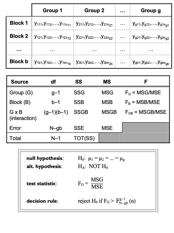
Two-way ANOVA is a method for “simultaneously” analyzing two factors that affect a response.

It is also called a “randomized block design”.

<Assumptions>

• Similar to the one-way ANOVA - normality, variance homogeneity.

<Test Setting>

<Takeaways>

• Another identifiable source of variation called a “blocking factor” is included in the model, whose variation can be separated from the error variation to give more precise group comparisons.

• The F-test for “group” (FG) tests the primary hypothesis of no group effect.
• F-test for the block effect (FB) provides a secondary test.

• Significant block effect often results in a smaller error variance (MSE) and greater precision for testing the primary hypothesis of no group effect, compared to the case where the block effects were ignored (but not always!).

• “Group-by-Block factor” (G x B) represents the statistical interaction between the two main effects. This indicates that trends across groups differ among the levels of the blocking factor.

• Interaction effect is usually the first test of interest in a two-way ANOVA model because the test for group effects might not be meaningful in the presence of a significant interaction.

• For the unbalanced groups (possibly due to missing data), sum of squares calculation is not trivial as it cannot be broken down into additive components due to the sources of variation. One way to address this issue is by using “weighted squares of means“.
• A statistical model associated with a higher-order ANOVA is called a fixed-effects model if all effects are fixed, a random-effects model if all effects are random, and a mixed effect model for a mixture of fixed and random effects.

 

---

5. Linear Regression

Linear Regression is used to analyze the relationship between a response variable $y$, and predictors $x$.

<Assumptions>

• Normality of the response
• Linearity between predictor and response
• Homoscedasticity: constant residual variance over the experimental region
• No autocorrelation (correlation over time)
• No multicollinearity: no redundant information in the predictors

<Test Setting>

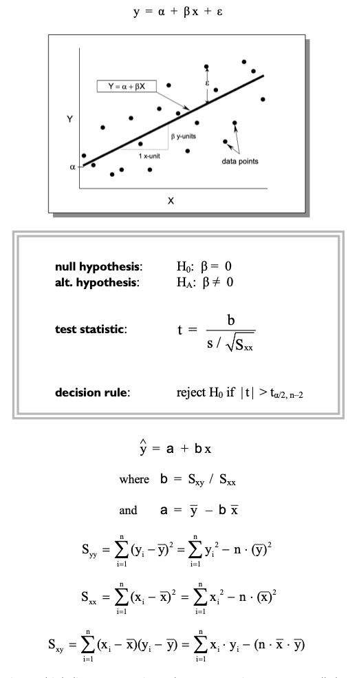
cf) for the case of multivariate predictors $\mathbf{X}$ (i.e. multiple linear regression), above expressions can naturally be extended to vector dimension. Namely, the best estimator of coefficients and intercept can be attained by solving the normal equation:

$$ \mathbf{\hat \beta} = (X^TX)^{-1}X^Ty $$

 

<Takeaways>

• As its name implies, “linear” regression models can only capture linear relationship between response and predictors. For other types of relationship (e.g. quadrature), we have to expand the model to include polynomial terms as well.

• The hypothesis of “zero regression slope” is equivalent to the hypothesis that the “covariate is not an important predictor of response”.

• For the multivariate case (i.e. multiple linear regression), coefficient of determination (R^2) represents the percentage reduction in error variability by using the explanatory variables as predictors of $y$ over just using the mean $\bar y$. This metric can be used for model (feature) selection.
• The fitted regression line can be used to “predict” the value of response given a new predictor.
• However, predicting a response outside the experimental region should be done with extra care as there is no guarentee that the same linear relationship will be held valid (a.k.a. extrapolation).
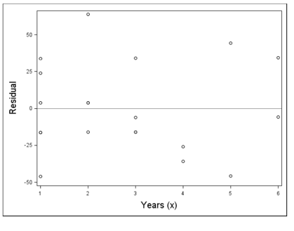
• To roughly diagnose the homoscedasticity assumption, we can use residual plot which is standardized residuals plotted against the predicted values of the response. Ideally, there should be no pattern like the one following:

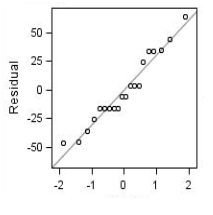
• For diagnosing the normality assumption, we can draw a normal qq plot :

• For diagnosing if autocorrelation exists, there is a test called Durbin-Watson test.
• Diagnostics available for detecting collinearity between independent variables include the variance inflation factor (VIF) and eigenvalue analysis of the model factors. For VIF approach, a widely used threshold is 10 (smaller the better).

 

---

6. Analysis of Covariance

Analysis of Covariance (ANCOVA) is used to compare response means among two or more groups “adjusted” for a quantitative concomitant variable (a.k.a. covariate), which is considered to have influenced the response.

<Assumptions>

• groups are independent
• normally distributed response measure
• variance homogeneity

<Test Setting>

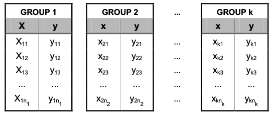
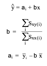
The mean response within each group depends on the covariate, which results in a model for the ith group mean as $\mu_i = \alpha_i + \beta x$. Then, the estimated regression line for $i$-th group is:

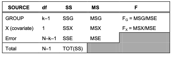
Similar to that of ANOVA, we can decompose the source of variation by the following table:

In this setting, our primary interest is the comparison of the group means adjusted to a common value of the covariate such that (little subscript 0 indicates covariates used):

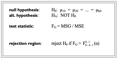
This hypothesis is equivalent to the “equality of intercepts among groups”, as each of the group means are only different in $\alpha$’s. Thus, the test does not depend on the value of covariate $x_0$.

$$ H_0: \alpha_1 = \alpha_2 = \dots = \alpha_k $$

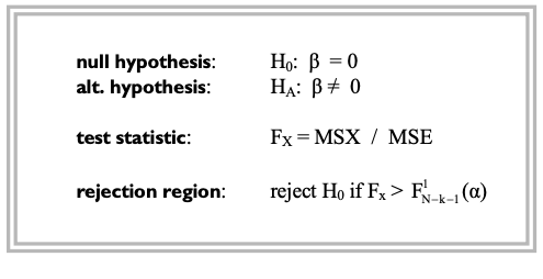
To determine whether the covariates have a significant effect on the response, use the $F_X$ ratio to test for zero-regression slope using the following test statistic:

<Takeaways>

• Basically, ANCOVA is combining regression and ANOVA methods by fitting simple linear regression models within each group and comparing regressions among groups. Therefore, the nitty-gritty details such as model intepretation and diagnosis follow that of the aformentioned two statistical models.

• ANCOVA can often increase the precision of comparisons of the group means and thereby decrease the estimated error variance, as the covariates can be a major source of variation among groups.
• Roughly speaking, the estimated effect among groups are shrunken towards the global mean of the model. This is often called as the “regression towards the mean”.

 

---

7. Wilcoxon Signed-Rank Test

Wilcoxon Signed-Rank Test is a non-parametric analog of the one-sample t-test.

<Assumptions>

• symmetrical underlying distribution
• No distributional assumptions as it is a non-parametric test.

<Notations>

• $y_1, y_2, \dots, y_n$: $n$ non-zero differences or changes (zeros are ignored)

• $R_i$: absolute rank of

  yi

  (in ascending order)

• $R_{(+)}$: the sum of the ranks associated with the “positive” values of the $y_i$’s
• $R_{(-)}$: the sum of the ranks associated with the “negative” values of the $y_i$’s

<Test Setting>

For a parameter θ which might represent the unknown population mean, median, or other location parameters, the test is defined as:

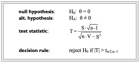
• Note that when $H_0$ is true, the test statistic $T$ has an approximate student-t distribution with $n–1$ degrees of freedom.

When there are tied data values (values are equal), the averaged rank is assigned to the corresponding $R_i$ values. If this is the case, we need a minor remedy in the calculation of $V$. To illustrate, suppose there are $g$ groups of tied data values. For the $j$-th group, compute $c_j = m(m-1)(m+1)$, where $m$ is the number of tied data values for that group. Then for the correction factor $C = c1 + c2 + \dots + c_g$,

$$ V = \frac{1}{24} \Big(n(n+1)(2n+1) - \frac{C}{2}\Big) $$

 

<Takeaways>

• So in a nutshell, this test is used to make inferences about a population mean or median without requiring the assumption of normally distributed data.
• Allbeit no requirement of distributional assumptions is clearly an advantage, the t-test is still more preferred for the following reasons:
  • t-test has been shown to have more statistical power in detecting true differences when the data are normally distributed.
  • Analysts often feel more comfortable reporting a t-test whenever it is appropriate, especially to a non-statisticians.
  • t-test is robust under deviations of its underlying assumptions. For example, the Central Limit Theorem guarentees asymptotic normality for the sample mean as long as we have large enough data.
  • In fact, Wilcoxon signed-rank test and t-test become closer as the sample size n gets larger.
• When the data are highly skewed or otherwise non-symmetrical, an alternative to the signed-rank test, such as the sign test (to be discussed in a second), can be used.

 

---

8. Wilcoxon Rank-Sum Test

Wilcoxon rank-sum test is a non-parametric analog of the two-sample t-test.

<Assumptions>

• Two population distributions have the same shape and differ only by a possible shift in location (i.e. variance homogeneity).

<Notations>

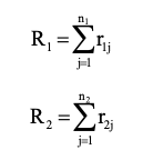
• $y_{(1,1)}, y_{(1,2)}, …, y_{(1,n_1)}$: independent samples in group 1 (total of $n_1$)
• $y_{(2,1)}, y_{(2,2)}, …, y_{(2,n_2)}$: independent samples in group 2 (total of $n_2$)
• $r_{(1, j)}$ : rank of $y_{(1, j)}, \quad (j=1, 2, … , n_1)$
  • data are ranked from lowest to highest over the combined samples
• $r_{(2, j)}$ : rank of $y_{(2, j)}, \quad (j=1, 2, … , n_2)$

<Test Setting>

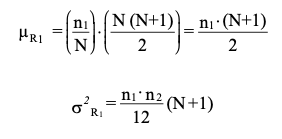
When $H_0$ is true, we would expect the proportion of the rank sum from group 1 to be about $n_1 / N$ and the proportion from group 2 to be about $n_2 / N$.

Hence, the expected value and variance of $R_1$ under $H_0$ is:

For tied values,

It has been shown that normal approximation to the Wilcoxon rank sum test is quite excellent even for samples as small as 8 per group in some cases.

Thus, for a location parameter θ, the test statistic is defined based on an approximate normal distribution such that:

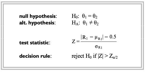
• cf) we can of course, use the exact Wilcoxon rank sum test using Wilcoxon rank-sum exact probabilities.

 

<Takeaways>

• This test is used to compare location parameters, such as the mean or median between two independent populations “without the assumption of normality”.

• It was originally developed for use with continuous numeric data. But it can also be applied to the analysis of ordered categorical data as well.

• For skewed distributions with long tails to the right (i.e. positively skewed), the median is usually smaller than the mean and considered a better measure of the distributional “center” or location.

• Mann-Whitney U-test is another non-parametric test for comparing location parameters based on two independent samples. Mathematically, it can be shown that the Mann-Whitney test is equivalent to the Wilcoxon rank-sum test.

• Wilcoxon rank-sum test is roughly equivalent to the two-sample t-test on the ranked data (Conover 1981).

 

---

9. Kruskal-Wallis Test

The Kruskal-Wallis test is a non-parametric analogue of the one-way ANOVA, which is used to compare population location parameters among two or more groups based on independent samples.

<Test Setting>

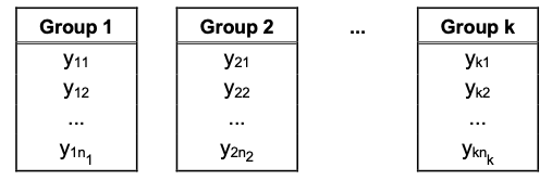
• The data are ranked, from lowest to highest, over the combined samples.

For $i = 1, 2, … , k$ and $j = 1, 2, …, n_i$, let $r_{(i, j)}$ =rank of $y_{(i, j)}$ over the $k$ combined samples.

For each group ($i = 1, 2, …, k$), compute:

$$ R_i = \sum_{j=1}^{n_i}r_{ij} $$

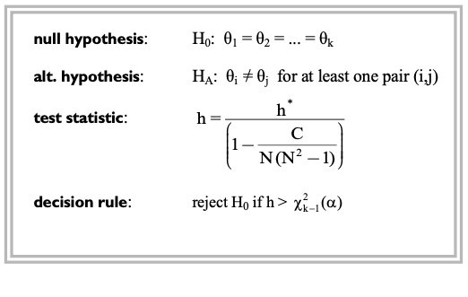
• when the null hypothesis is true (i.e. no difference between average responses), the average rank for each group, namely $R_i / n_i$, should be close to $\bar R = (N+1) / 2$, where $N = n_1 + n_2 + \dots + n_k$. Also the following sum-of-squared deviations should be small.

$$ \sum_{i=1}^k n_i \big( \bar R_i - \bar R \big)^2 $$

In this setting, the Kruskal-Wallis test statistic is a function of this sum of squares, which can be simplified as the following formula:

$$ h^* = \frac{12}{N(N+1)} \Big( \sum_{i=1}^k \frac{R_i^2}{n_i} \Big) - 3(N+1) $$

When $H_0$ is true, $h^*$ has an approximate $\chi^2$ distribution with $k–1$ degrees of freedom, which completely defines the test.

Under the existence of tied values, a minor adjustment to the test statistic is made such that for the number of tied values for $L$-th category $m$,

<Takeaways>

• Kruskal-Wallis test can also be seen as an multivariate extension of the Wilcoxon rank-sum test. Specifically, when $k=2$, the Kruskal-Wallis chi-square value has 1 degree of freedom. Then the test is identical to the normal approximation used for the Wilcoxon rank-sum test such that the h-statistic is the square of the Wilcoxon rank-sum Z-test.
• The effect of adjusting for tied ranks is to slightly increase the value of the test statistic h. Therefore, omission of this adjustment results in a more conservative test.

• When the Kruskal-Wallis test is significant, pairwise comparisons can be carried out using the Wilcoxon rank-sum test for each pairs of groups (although multiplicity of the test has to be addressed).

• When the $k$-levels of the Group factors can be “ordered”, we might want to test for association between response and increasing levels of group. The Jonckheere-Terpstra test can be utilized for this purpose.

$$ H_A: \theta_1\leq \theta_2 \leq \dots \leq \theta_k $$

 

---

10. Binomial Test

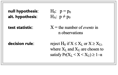
The binomial test is used to make inferences about a proportion or response rate based on a series of independent observations, each resulting in one of two possible mutually exclusive outcomes represented as binary indicator variable.

<Test Setting>

• $n$ independent observations, each with one of two possible outcomes: event or non-event.

• For each observation, the probability of the event is denoted by $p, \quad (0 < p < 1)$

• The total number of events in $n$ observations $X$, follows the binomial distribution with parameter $p$. Thus $X = np$.
• A natural estimator of the population success probability $p$ is the sample proportion $X / n$. In fact, this is the MLE of the natural parameter.

<Takeaways>

• By the CLT, a binomial response $X$ (number of success in $n$ trials) has an asymptotic normal distribution. Specifically, it approaches normal distribution with mean $np$ and variance $n^2 p(1–p)$.

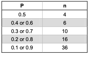
• The normal approximation to the binomial is generally a good approximation if:

$$ \begin{aligned} n \geq 4 \times \text{max}\Big\{(p/(1-p), (1-p)/p \Big\} \end{aligned} $$

• When $p_0 = 0.5$, the binomial test is sometimes called as the sign test.

 

---

11. Chi-Square Test

The chi-square test is used to compare two independent binomial proportions, $p_1$ and $p_2$.

<Assumptions>

• Two groups are independent.
• normal approximation to the binomial distribution is valid.

<Test Setting>

Observations are made of $X_1$ responders out of $n_1$ subjects whom are studied in the first group, and $X_2$ responders out of $n_2$ subjects in the second group. Note that both groups are independent.

Assume that each of the $n_i$ subjects in $i$-th group ($i =1, 2$) have the same chance $p_i$ of responding, so that $X_1$ and $X_2$ are independent binomial random variables.

In this setting, the goal is to compare population response rates between two groups (i.e. $p_1 \text{ vs } p_2$).

Assuming that the normal approximation to the binomial distribution is valid, test is defined as the following:

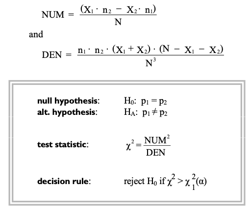
Note that the chi-square statistic can be re-expressed as:

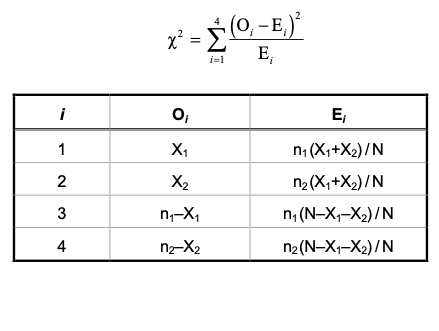
<Takeaways>

• chi-square test is an approximate test, which may be used when the normal approximation **to the binomial distribution is valid. If this approximation is not guarenteed, an alternative approach is the **Fisher’s exact test which is based on exact probabilities (to be discussed in a second).
• As the square of a standard normal random variable is defined as a chi-square random variable with 1 degree of freedom, it can be shown algebraically that the chi-square test is equivalent to the Z-test when comparing only two binomial proportions.

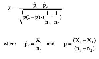
• The approximate 95% confidence interval for the difference in proportions, $p_1 – p_2$ is given by:

 

---

12. Fisher’s Exact Test

The Fisher’s exact test is an alternative to the chi-square test for comparing two independent binomial proportions $p_1$ and $p_2$.

Specifically, it is useful when the normal approximation to the binomial might not be applicable, such as in the case of small cell sizes or extreme proportions.

<Assumptions>

• Two groups are independent.

<Test Setting>

Observations are made of $X_1$ responders out of $n_1$ subjects whom are studied in the first group, and $X_2$ responders out of $n_2$ subjects in the second group, both groups are independent (same as that of chi-square test).

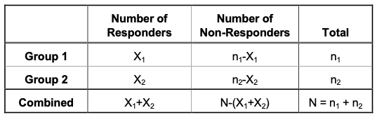
Given equal proportions $p_1 = p_2 (\because H_0)$, the probability of observing the configuration shown in the above table (marginal totals $n_1, n_2$ are fixed) is derived by the “hypergeometric distribution” with probability:

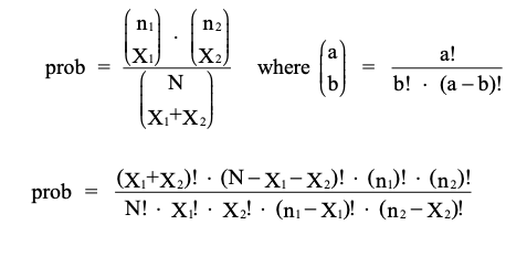
Under this setting, the p-value for the test (i.e. Fisher’s exact probability) is the probability of the observed configuration plus the sum of the probabilities of all other configurations with a “more extreme result” for fixed row and column totals.

<Takeaways>

• So basically, in order to use this test, we have to compute all the possible combinations of the configurations which takes huge amount of time and effort.

• For this reason, although Fisher’s exact test is valid no matter how large the sample size is, its usage is most often limited for small cell frequencies.

• Fisher’s exact test can be extended to situations that involve more than two treatment groups or more than two response levels. This is sometimes referred to as the generalized Fisher’s exact test or the Freeman-Halton test.

 

---

13. McNemar’s Test

The McNemar’s test is a special case of comparing two binomial proportions for paired samples.

Paired samples are often collected in a clinical trials where dichotomous outcomes are recorded for each patient under two different conditions (e.g. before/after treatment is applied), and the goal is to compare response rates under the two sets of conditions or matched observations.

Note that in these cases, the assumption of independence among groups is not met, so we cannot use the chi-square test or Fisher’s exact test.

<Assumptions>

• normal approximation to the binomial distribution is valid.

<Test Setting>

There are $n$ pairs of observations, each observation in the pair resulting in a dichotomous outcome, say “response” or “non-response”.

Considering all possible scenarios user this problem setting, the results can be partitioned into 4 subgroups such that:

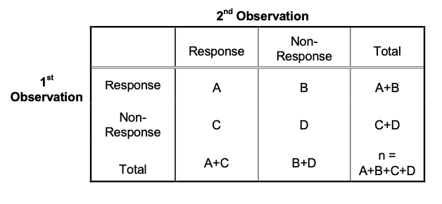
Let $p_1$ represent the probability that the first observation of the pair is a ‘response’, and $p_2$ the probability that the second observation is a ‘response’.

Then, the hypothesis of interest is the equality of the response proportions (i.e. $p_1$ = $p_2$), and the test statistic is constructed based on the difference in the “discordant” cell frequencies (B and C in above table) which follows $\chi^2$ distribution with 1 degrees of freedom under $H_0$.

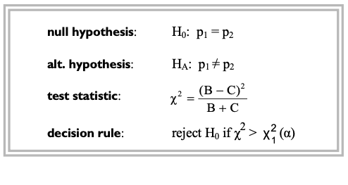
<Takeaways>

• In above setting, the natural estimate of $p_1$ is $\frac{A + B}{n}$, and that of $p_2$ is $\frac{A + C}{n}$.
• The difference in proportions $p_1 – p_2$ is estimated by $\frac{A + B}{n} – \frac{A + C}{n} = \frac{B – C}{n}$.
• An approximate 95% confidence interval for $p_1 – p_2$ is:

• Note that the $\chi^2$ test statistic is based only on the discordant cell sizes (B, C) and ignores the concordant cells (A, D). However, the estimates of $p_1, p_2$ and the size of the confidence interval are based on all cells, as they are inversely proportional to the total sample size $n$.

• By the normal approximation of binomial random variable, it can be shown that McNemar’s test is equivalent to the binomial test with $H_0: p = 0.5$, where $p$ equals the fraction of the events that fall in one of the discordant cells (when $H_0$ is true, the discordant values B and C should be about the same so $\frac{B}{B+C} \approx 0.5$).
• Thus, with $n = B + C$ and $X = B$,

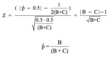
• The condition for normal approximation is (need to be checked only if either B or C is less than 4):

$$ \begin{aligned} \big\{B^2 \geq C(4-B)\big\} \cup \big\{ C^2 \geq B(4-C) \big\} \end{aligned} $$

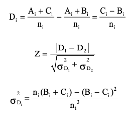
• McNemar’s test is often used to detect shifts in response rates between pre- and post-treatment measurements within a single treatment group such that (under the null hypothesis of no difference in shifts between groups):

 

---

14. Cochran-Mantel-Haenszel Test

The Cochran-Mantel-Haenszel test is used to compare two binomial proportions from independent populations based on stratified samples.

In clinical trials, it is often used in the comparison of response rates between two treatment groups in a multi-center study using the study centers as strata.

<Test Setting>

There are $k \geq 2$ strata with for a single stratum $j$, exists $N_j$ patients $(j = 1, 2, …, k)$, randomly assigned to one of two groups.

In the first group, there are $n_{(j, 1)}$ patients with $X_{(j, 1)}$ of whom are considered “responders”. Similarly, the second group has $n_{(j, 2)}$ patients with $X_{(j, 2)}$ “responders”, as in the following table:

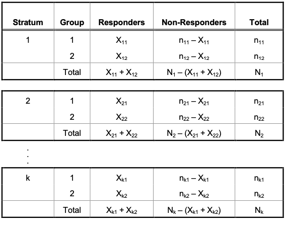
Let $p_1, p_2$ denote the overall response rates for Group 1 and Group 2 respectively. For the $j$-th stratum, compute the quantities:

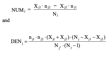
Then, the Cochran-Mantel-Haenszel test is defined as the following:

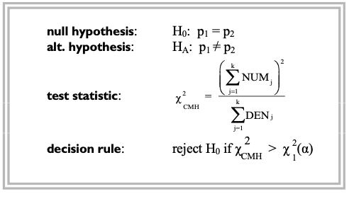
<Takeaways>

• The stratification factor can represent patient subgroups such as “study centers”, “gender”, “age group”, or “disease severity” and acts similar to the “blocking factor” in a two-way ANOVA
• It obtains an overall comparison of response rates “adjusted” for the stratification variable. The adjustment is simply a weighting of the 2×2 tables in proportion to the within-strata sample sizes.
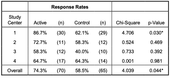
• A convenient way to summarize the test results by stratum is providing a summary table such that:

• The overall response rate for Group $i$ is estimated by $100 \times (\frac{X_{1i} +X_{2i} +X_{3i} +X_{4i}}{n_{1i} +n_{2i} +n_{3i} +n_{4i}})$ %

• This Cochran-Mantel-Haenszel test can often be useful when there is a big difference in sample sizes among strata and the largest strata showing the biggest response rate differences.

• Cochran-Mantel-Haenszel statistic can be understood as to be based on the within-strata response rate differences combined over all strata with some weight applied. Specifilly, the weight is:

$$ w_j = \Big( \frac{1}{n_{j1}} + \frac{1}{n_{j2}} \Big)^{-1} $$

• Although the derivation is omitted here, to get a glimpse of what’s happening, greater weights are assigned to those strata that have larger sample sizes.

 

---

15. Logistic Regression

Logistic regression analysis is a statistical modeling method for analyzing categorical response data while accommodating adjustments for one or more explanatory variables, namely “covariates”.

<Assumptions>

• no interaction effects among covariates (equal slopes of the logit function among groups).
• covariance structure of the response variable is held constant.

<Test Setting>

Suppose we have $N$ subjects with $k$ covariates $X_1, X_2, \dots, X_k$. Also, the response $y$ is a binary indicator (1: event // 0: non-event).

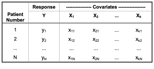
Since the response is confined in the probability interval between $[0, 1]$, we apply the logit link function to the response variable $y$ to statistically connect it to the linear combination of the covariates.

In this setting, the model for the probability of “event“, say $P$ is:

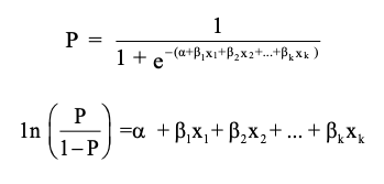
, where the latter expression is in terms of log odds ratio.

If all the $X$’s are continuous numeric covariates, the odds can be expressed as:

, with the odds ratio for Xi is $\text{OR}_{x_i} = \text{exp}(\beta_i)$.

The interpretation of this odds ratio is to see the percentage increase in the odds of “event” occurrence when $X_i$ increases by 1 unit and all other $X$’s are held constant (i.e $100 \times (\text{exp}(\beta_i)-1)$)

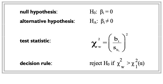
Then, the test becomes equivalent to see if a particular regression coefficient $\beta_i$ is statistically significant is based on the Wald (chi-square) Test.

<Takeaways>

• It closely resembles the idea of linear regression and ANCOVA models, but the main difference is in the target variable to be applied such that logistic regression analyzes proportions based on categorical responses (most commonly binary responses).
• For the purpose of seeing the “equality of response rates between groups” usually expressed as the hypothesis of a zero difference, we can compare response rates by measuring how close the odds ratio is to “1”. This ratio is called “relative risk“ and as the odds ratio gets closer to the relative risk, the event becomes more rare.
• We can compare the relative importance of covariates measured on different scales by standardizing the $\beta$ estimates by dividing by their standard errors.

 

---

Reference

• Walker, G., & Shostak, J. (2010). Common statistical methods for clinical research with SAS examples. SAS institute.